Introduction

Since Daniel Bernoulli used a mathematical method in 1766 to evaluate the effectiveness of variation until today, a large number of models and mathematical-epidemiological concepts have been developed to study and follow the behavior of different infectious diseases in the population. Numerous authors such as J. Brownlee (1906, 1918), R. Ross (1911, 1917), McKendrick and Kermack (1927), and Reed and Frost (1928), among others, contributed to the development of this area of ​​knowledge[1]. Later there was great development that included the spatial dimension, seasonality and the role of carriers, venereal transmission and others. Among these, the contributions of Anderson and May (1978), of Hudson and Dobson from 1985 onwards, and of Roberts and Grenfell from the 90’s[1] stand out. A large number of studies highlighted concepts such as threshold population, herd immunity[2],[3],[4],[5], reproductive number, serial interval, incubation times, and spillover in the dynamics of infectious diseases. All of these concepts contribute in some way to decision-making[6],[7],[8]. In recent decades emphasis has been placed on spatial propagation[9],[10],[11],[12],[13],[14],[15],[16],[17], the role of population mobility, and the connectivity of transportation networks such as airlines during the spread of epidemics[18],[19],[20],[21],[22],[23]. These models have made great contributions to the study of different diseases such as Influenza AH1N1, AH5N1, HIV, SARS, and Ebola[18],[19],[20],[21],[22].

Numerous models have been developed for the current COVID-19 pandemic, a disease caused by the SARS-CoV-2 virus, and for SARS[24],[25],[26],[27]. Most correspond to Susceptible-Exposed-Infected-Removed (SEIR) models with different stratification types, be it spatial, age, socio-economic, etc. Given the great complexity of forms of spreading, mathematical models can offer valuable tools to synthesize information to understand epidemiological patterns and develop quantitative evidence to inform global health decisions [6].

A model has been used in Chile with good success to short-term forecast ICU occupancy, warning authorities of the possible collapse of hospital capacity[28]. SEIR-type models are also used to predict the evolution of the epidemic locally[29]. Another study uses a polynomial cubic adjustment model to estimate case number and an exponential total case model to represent the daily effort to reduce the initial daily growth rate to warn of the pandemic’s potential[30]. Another study also analyzed the minimum daily effort required for the healthcare system to not collapse during the COVID-19 outbreak. A parametric threshold condition is obtained, which involves a parameter associated with the minimum daily effort for not collapsing the system[31]. All studies have helped to highlight the importance of modeling in decision-making[32].

The COVID-19 pandemic has cost more than 12 000 deaths in Chile. Initially, it had an accelerated growth that was partially controlled with interventions, such as closing schools and universities and implementing partial quarantines. After these initial measures, a relaxation of interventions and late interventions led to a large epidemic mainly concentrated in the Metropolitan Region (Santiago), despite the warnings made by the scientific community and different epidemic modeling teams. Subsequently, massive quarantines were established that have been associated with a decrease in the number of cases, leading to a relatively stable number, between 1 000 and 2 000, of daily cases in the country[33]. Throughout this process, a series of factors have complicated the follow-up of cases, such as changes in the notification system and underreporting cases.

Considering that the simplest models can significantly contribute to the monitoring and prediction of epidemics, we have developed three simple mathematical approaches to understand and monitor the dynamics of the COVID-19 pandemic and contribute to decision-making in Chile. In this contribution, we report and discuss the usefulness, the successes, and the practical difficulties that have transpired in the development of COVID-19.

Methods

We carried out an ecological study using official daily public reports from the Chilean Ministry of Health, including new confirmed cases, cases that required admission to the ICU, and deaths attributable to COVID-19 nationally and sub-nationally (regions). With this information, we made: 1) estimates of the effective reproductive number Rt; 2) estimates of the underreporting of cases; and 3) we developed three models with different objectives to follow the epidemic in Chile.

We calculate Rt using the method developed by Cori et al[34]. We consider the last two weeks (14 days) and a serial interval τ = 5 days with variability between 2 and 8 days (based on[35],[36],[37]). The underreporting of cases was estimated according to the method proposed by Russell et al. [38],[39] adapted to the situation in Chile[33].

Maximum potential load model
The objective of this model has been to follow the evolution of the epidemic curve and establish short-term predictions (1 week) of the maximum potential loads of new cases, ICU occupancy, and deaths. This seeks to estimate the health system’s saturation level, which would allow informing decisions that aim to reduce the number of infections or increase the health system’s response capacity.

If there are C_t new cases in a week “t” and that there are I_t = (C_t + C_t-1) infected people, considering that the cases remain contagious for up to two weeks, it can be proposed that: 

C_t+1 ≈ R_t (C_t + C_t-1).

This means that all those infected in the previous two weeks are contagious and will contribute to infections the following week. However, not all infected individuals on a day “i” will become cases the following week, as this depends on the serial interval and its probability distribution. A more suitable expression is:

, t in weeks, i in days, where tf represents the last day of the week “t”, p_i represents the probability that someone infected on day “tf-i” infects someone in week t + 1. Thus a better expression is:

C_t+1 ≈ fR_t (C_t + C_t-1) (1).

where f corresponds to a correction factor as a consequence of the probability distribution of the serial interval. For a maximum load, the correction factor is estimated as the maximum p_i (i = 0-13) for a Gamma distribution with mean 5 and standard deviation 4.3 days (based on[35],[36],[37]); the correction factor is f ≈0.8. The equation (2) is a Fibbonacci like series, and requires two initial conditions (t₁ and t₂). In this study these was t₁ = 10 (March 8), t₂ =65 (March 15)(the new cases in the two first weeks).

Considering that approximately 3.5% of the cases reach an ICU (0.035Ct), that on average, an ICU is occupied for approximately two weeks, and that the latency between onset of symptoms and ICU requirement is approximately one week[38],[39], it can be proposed that occupied ICUs (U_t):

U_t+1 = 0,035 (C_t + C_t-1) (2).

To estimate the maximum number of deaths (Dt), we consider a latency of two weeks between the onset of symptoms and death of symptomatic patients of 2.6%[38],[39]. So:

D_t+1 = 0.026T_t-1 (3)

where T_t-1 corresponds to the total number of cases from two weeks ago. Thus equations (1), (2) and (3) constitute the basis of this model. This model allows to predict the maximum potential load of COVID-19 expected for the following week, based on the “history” of the two previous weeks.

Discreet SEIR model and stochastic model
The objective of this model has been to try to predict the shape of the epidemic curve and the times in which the increase in the number of cases, the peak, and the decrease would occur in the earliest possible way. We use a variation of a SEIR (Susceptible (S), Latent (E), Infectious (I), removed (deceased + recovered (Rm)) model in its discrete form:

S_i+1 = S_i – βS_iI_i (4).

E_i+1 = E_i + βS_iI_i  – νE_i (5).

I _i+1 = I _i + νE_i – (μ + γ) I_i (6).

Rm_i+1 = Rm_i + (μ + γ) I_i (7).

C_i+1 = pI_i (8).

U_i+1 = qC_i-7 (9).

D_i+1 = hT_i-14 (10).

Where β is the transmission coefficient, ν the transfer rate from E to I, µ the mortality rate, γ the recovery rate, p the proportion of infected who are notified, q the proportion of symptomatic patients requiring ICU and h the fatality rate. The sub-idex “i”represents time in days. In this study the parameters ν = 1/5 days^-1, (µ + γ) = 1/14 days^-1, p = 0.1, q = 0.035 and h = 0.026 were considered constant and the transmission coefficient β and the asymptote of the model "S*" as variable parameters. The model was adjusted as the epidemic progressed, depending on the changes in the number of reported and in the notification system. Initially, on April 15, the asymptote of the model “S*” was estimated considering a Chilean population of 19,000,000, a proportion of herd immunity 57.4%, that 5% could get sick (based on European experience), and a heterogeneity correction factor of 0.5 considering that at this time the epidemic was centered in Santiago. Thus initial S* = 19,000,000 x 0.547 x 0.5 x 0.05 = 259,825 cases. The transmission coefficient β was estimated adjusting the best model. The model was adjusted weekly (if necessary), varying S* and β. The goodness of fit of the model was studied with the coefficient of determination (R²) and its significance (F-test).

Given the great variability and stochastic fluctuations of the cases worldwide, in order to include their effects on the dynamics, we consider the simple stochastic version of the previous model, with the same parameters, based on equations (4) to (7), with the Monte Carlo kinetic method with the Gillespie algorithm[40]. In this, we consider the three events:

1. A latent occurs with rate a₁: βS(i)I(i); S = S-1; E = E+1;
2. An infected occurs with rate a₂: νE(i); E =E-1; I = I+1
3. A removed occurs with rate a₃: (μ + γ)I(i); I =I-1; Rm =Rm+1

The probability for a_j is: . The time until the next event (τ) is exponentially distributed, with a rate equal to the sum of the rates of all possible events: f(τ) = ∑ _jα _je^{-τ∑ jaj} with an expected value  [39].

Gompertz model
When a flattening in the curve of the total cases could already be established in Santiago, a generalized logistic type model, the Gompertz model, was fitted to the curve of the total cases (T(t)):  (11), where A is the asymptote and b and c are the parameters that control the curve’s position and the growth rate, respectively[41].

Results

Maximum potential load model
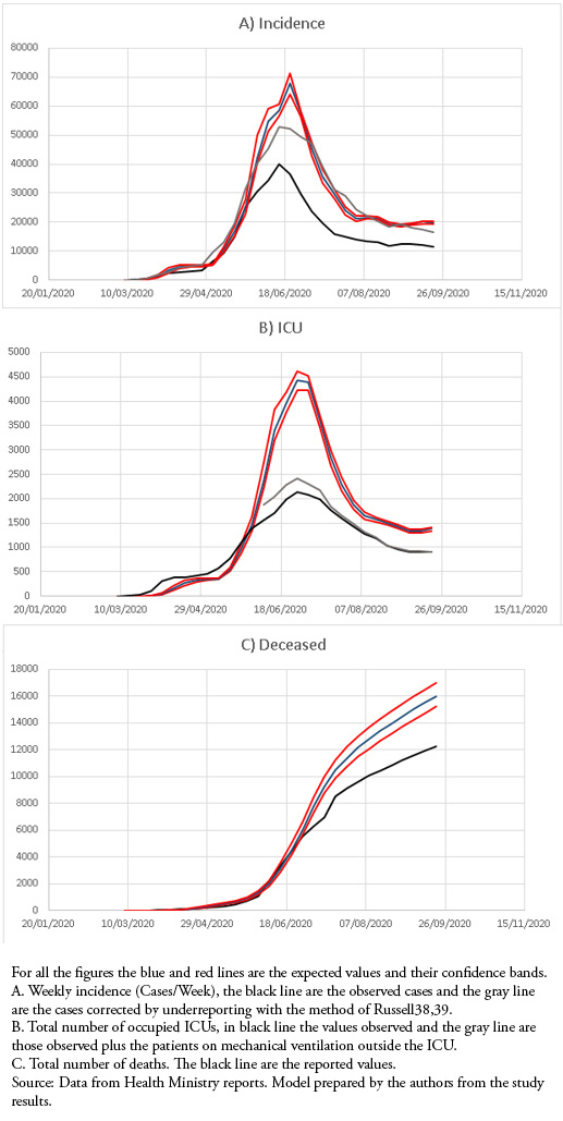
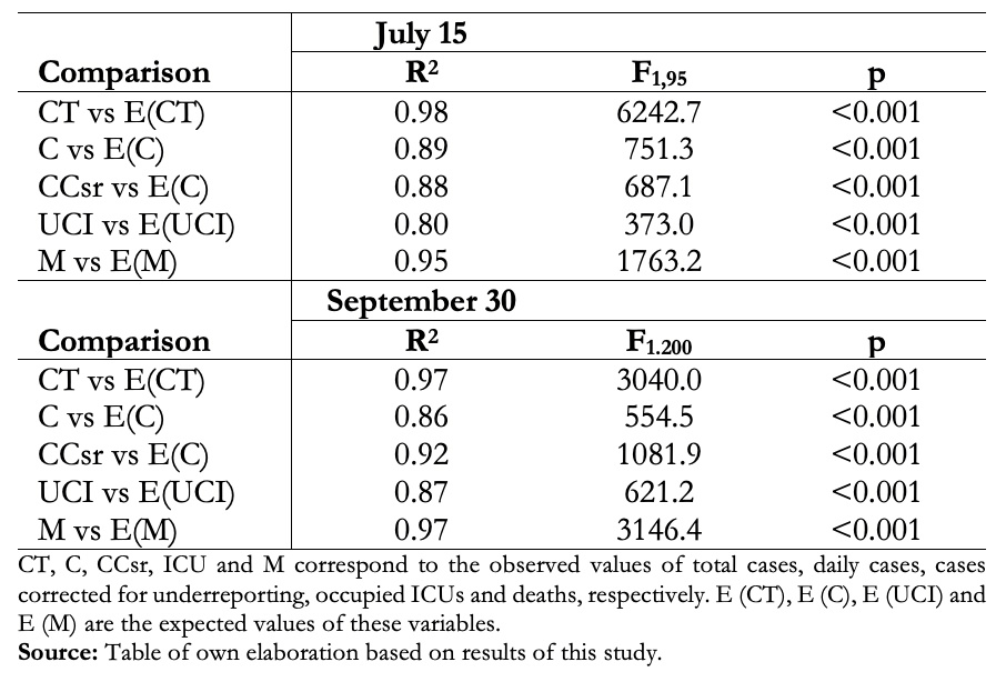
This model adequately reproduced the shape of the epidemic curve, maintaining values above those observed for weekly cases, the number of occupied ICUs, and the total number of deaths. When weekly cases were corrected for underreporting, they approached the maximum load predictions (Fig 1).

Figure 1.

Discrete model of maximum potential load.

Full size

Discrete SEIR Models and Stochastic Model
This model was very useful in predicting the rise, peak, and decline of cases, with great predictive power until the decline phase of the initial outbreak in July and early August. (Fig 2A, Table 1). In recent months there has been a better adjustment to the corrected cases, but it has been losing adjustment, especially in ICUs and the number of deaths, which has had major changes in the reporting system (Fig 2B, Table 1). The stochastic SEIR model allowed us to observe whether the variations in the number of cases were due to a mismatch in the model or to random fluctuations (Fig. 2C).

Table 1.

Adjustment of the deterministic SEIR model to the observed values.

Full size

Figure 2.

Discrete deterministic SEIR model.

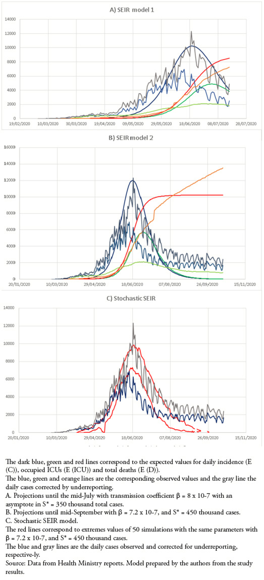Full size

Gompertz Model for the Metropolitan Region (Santiago)
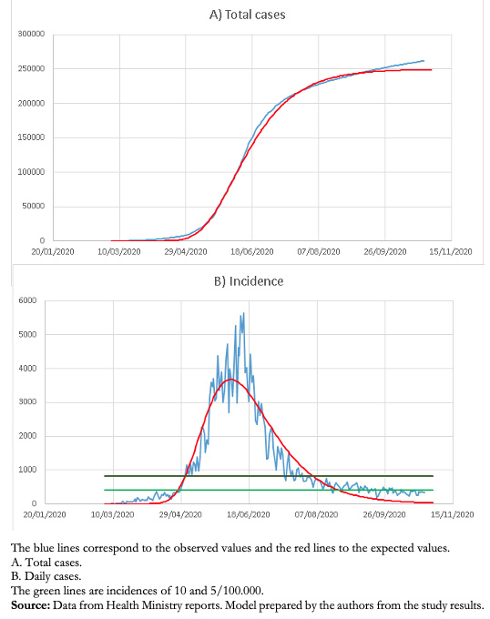
This model has allowed a good follow-up of the decrease in the number of cases in the Metropolitan Region and, so far, an adequate prediction of the endemic situation (Fig. 3).

Figure 3.

Gompertz models for the Metropolitan Region (Santiago).

Full size

Discussion

Mathematical models play an important role in monitoring epidemics, helping to rationalize decision-making, and predicting important events in the course of epidemics, such as increase, peak, and decrease in incidence.

The objective of the maximum potential load model was to predict the maximum incidence, number of occupied ICUs, and deaths within a week. Initially, while the epidemic had very high reproductive numbers, greater than 1.5[33], the predicted values ​​were very similar and even lower than those ​​observed for ICU incidence and occupation. However, after May 30, the predicted values ​​had a higher limit than the observed values, allowing an adequate safety coefficient in the prediction. For incidence, when the number of cases was corrected for underreporting, which has varied between 30 and 60% throughout the epidemic[33], the values ​​were quite close to the predicted values ​​except for the maximum. The prediction of occupied ICUs in the maximum period was much higher than that observed, partly explained because there was a saturation of ICU capacity during the maximum period, with up to 400 patients on invasive mechanical ventilation outside the ICU. Up to now, the model has followed the morphology of the epidemic curves adequately, but its predictive capacity is short, only one week, which is similar to previous models developed for the AH1N1 epidemic in Chile[13],[14],[15].

The SEIR model was very adequate, with an excellent prediction of the rise, peak, and decline in the number of new cases. This model used several fixed parameters that are well justified. Latent period of 5 days[37], infectious period[38],[39], 3.5% ICU occupancy[42] and 2.6% fatality[38],[39]. In addition, considering 10% of new cases in relation to active cases was an adequate assumption, since currently, the percentage of new notified cases / active cases is 9.3 ± 4.9%. The transmission coefficient was empirically adjusted initially using 3.98 x 10^-8 in early April, predicting a maximum in early May; later, on April 15, it was adjusted to 8 x 10^-7 with an asymptote of 350 000 cases, with an excellent adjustment that predicted the maximum for June 19, which it occurred on June 14. It also had a good prediction for the initial decline in cases. Also, until the last week of June, it had an adequate prediction of the total number of deaths. However, the prediction of occupied was well above the number of occupied ICUs, partly explained by the saturation already mentioned. The decrease in the number of cases did not follow a typical curve of a SEIR model, which forced a new adjustment in July with β = 7.2 x 10^-7, with a load capacity of 450 000 cases, which improved the adjustment only for two weeks; later it lost all predictive capacity since the beginning of August. The stochastic SEIR model allowed for the inclusion of the variability of the predictions and showed the same loss of predictive capacity as the deterministic model.

The good predictive capacity of the number of cases and the date of occurrence of the maximum and also the loss of predictive capacity during the decline of the epidemic is explained because, during much of the epidemic, the rise in cases and the maximum number of cases were produced mainly by cases in the Metropolitan Region (which includes Santiago), a region that has a population of approximately eight million inhabitants, about 42% of the population of Chile. This population is highly intercommunicated, behaving as a unit. The decrease in the Metropolitan Region cases has coincided with the gradual and asynchronous rise in cases in the remaining 15 regions, which has kept the cases in a high endemic state (Figure 4).

Figure 4.

Evolution of the daily incidence of COVID-19 in Chile.

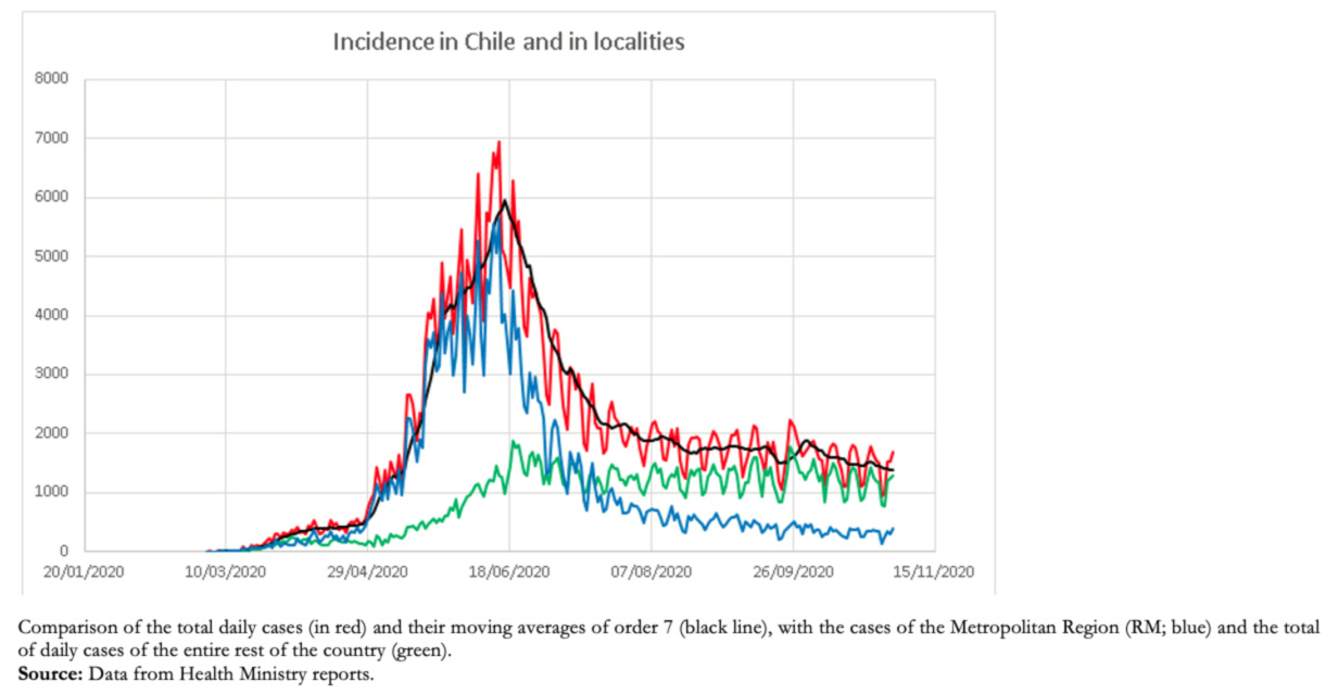Full size

As the decrease in the Metropolitan Region cases was asymmetric, a Gompertz model was fitted, which has shown a very good fit in much of the process; however, in recent days, it has also been losing predictive capacity. This is probably because the decrease in the number of cases has not occurred naturally due to herd immunity but instead associated with a series of interventions that have confined a large part of the population[33]. Currently, the Metropolitan region is relatively stable at lower than 10 cases per 100 000 inhabitants.

In summary, the models used have been very useful, with different objectives at different stages of the epidemic. The short-term model is still useful, providing an upper bound on the number of cases each week; the SEIR model had a very good predictive capacity of the maximum; the stochastic model introduced variability in the prediction, and the Gompertz model has had a better predictive capacity of the decline in cases.

Notes

Authorship contributions

Competing interests

Funding

Ethics 

From the editors