Methodological notes
← vista completaPublished on November 7, 2019 | http://doi.org/10.5867/medwave.2019.10.7716
General concepts in biostatistics and clinical epidemiology: observational studies with case-control design
Conceptos generales en bioestadística y epidemiología clínica: estudios observacionales con diseño de casos y controles
Abstract
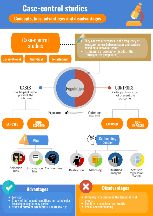
Case-control studies have been essential to the field of epidemiology and in public health research. In this design, data analysis is carried out from the outcome to the exposure, that is, retrospectively, as the association between exposure and outcome is studied between people who present a condition (cases) and those who do not (controls). They are thus very useful for studying infrequent conditions, or for those that involve a long latency period. There are different case selection methodologies, but the central aspect is the selection of controls. Data collection can be retrospective (obtained from clinical records) or prospective (applying data collection instruments to participants). Depending on the objective of the study, different types of case-control studies are available; however, all present a particular vulnerability to information bias and confounding, which can be controlled at the level of design and in the statistical analysis. This review addresses general theoretical concepts concerning case-control studies, including their historical development, methods for selecting participants, types of case-control studies, association measures, potential biases, as well as their advantages and disadvantages. Finally, concepts about the relevance on this study design are discussed, with a view to aid comprehension for undergraduate and graduate students of the health sciences. This is the third of a methodological series of articles on general concepts in biostatistics and clinical epidemiology developed by the Chair of Scientific Research Methodology at the School of Medicine, University of Valparaíso, Chile.
Main messages
- Case-control studies analyze associations between an exposure factor and an outcome in people in whom the condition is present (cases) or absent (controls).
- This design is useful for studying conditions that are infrequent, or those that require a long latency to occur. However, they are vulnerable to information bias and confounding.
Introduction
Elements of the case-control design have been evident since the nineteenth century. Perhaps the most well-known example is that of the cholera outbreaks investigated by John Snow and Reverend Henry Whitehead, ultimately leading to the discovery that the Broad Street water pump was the cause[1],[2]. Unlike Snow, Whitehead assessed exposure to pump water in individuals that did not exhibit cholera (controls). Through a thorough and systematic survey, which included visiting individuals up to five times, Whitehead collected basic but relevant information regarding water consumption among Broad Street residents, concluding that using water from a specific pump associated with cholera, a finding that resulted in a decrease from 127 deaths on September 2, to 30 on September 8, in 1854[3].
However, the modern conception of the case-control design is attributed to Janet Lane-Claypon for her work on risk factors associated with breast cancer (1926)[4]. In 1939, another case-control study led by Franz Müller[5], member of the Nazi party, linked the consumption of cigarettes with lung cancer, consistent with Hitler's position against smoking; indeed, his government promoted propaganda campaigns against tobacco consumption in light of recently available evidence. Müller sent a questionnaire to relatives of lung cancer victims, inquiring about consumption habits, including form, frequency, and type of tobacco used, corroborating a strong association between tobacco consumption and the disease[5],[6]. Subsequently, and parallel to the course of World War II, there was a halt in the development of this methodological design until four case-control studies were published in 1950. They all analyzed the relationship between smoking and lung cancer, validating the use of this design to determine the etiology of diseases. One of these was led by Richard Doll and Austin Bradford Hill[7],[8], who believed that increases in lung cancer rates in England and Wales could not fully be explained by improvements in diagnostic tests -as was argued at the time- but rather environmental factors including smoking and air pollution[7].
Decades later, in 1987, a study of risk factors associated with the transmission of Acquired Immunodeficiency Syndrome, such as promiscuity and the use of intravenous drugs[9],[10], enabled the implementation of measures that reduced transmission, even before the virus had been identified[10].
Thus, epidemiology shifted from determining causes to determining risk factors[1]; Snow was not interested in determining the causal agent but rather ways cholera was transmitted[3]. In this way, observational designs such as case-control and cohort studies are available to study etiology and prognostic factors (protective factors and risk factors)[11]. In this article, we will focus on the former, while cohort studies will be the subject of the next article in this series.
This review is the third of a methodological series comprising six narrative reviews that cover general topics in biostatistics and clinical epidemiology. The series is based on content from publications available from major databases of the scientific literature, as well as specialized reference texts. The series is oriented toward undergraduate and graduate students and is developed by the Chair of Scientific Research Methodology at the School of Medicine, University of Valparaíso, Chile. Therefore, the purpose of this manuscript is to address the main theoretical and practical concepts of case-control studies.
Preliminary concepts
Case-control studies constitute an observational, analytical and longitudinal design: the researcher does not assign exposures, the design permits hypothesis testing, and there is a period between exposures and outcomes. Some authors purport that causal relationships could be demonstrated through a case-control design[12]; however, this is controversial. To execute a case-control study, a group of participants similar in baseline characteristics are recruited that either present an outcome of interest (cases) or do not present it (controls). In both cases and controls, variables that represent risk factors are measured and compared between the two. Thus, a fundamental characteristic of a case-control study is that the subjects are selected according to an outcome; this is an advantage given it is not necessary to wait a prolonged period for the phenomenon under study to occur. It can also present a disadvantage as in most cases data will have to be collected retrospectively and quality will depend on an adequate record or participants’ memory[13].
Selection of cases
The selection of cases must be rigorous, privileging incident cases (cases that have been recently diagnosed) over prevalent cases (all available cases, including those diagnosed years prior). Incident cases are likely more similar in how they were diagnosed, and more consistent with the present diagnostic criteria.
It is thus necessary to have a clear definition of the outcome, for example, current and international diagnostic criteria, laboratory tests, imaging studies, among others. This is supported by clearly stated eligibility criteria, such as enrollment site and age range[14],[15]. Potential sources for cases include hospitals, communities or population registries, or patient groups, such as Alcoholics Anonymous or support groups such as those for specific genetic diseases. Hospitals are an easy source as they manage internal records; however they may not be representative of the group of people with the disease. On the other hand, population cases are more challenging to locate in the absence of registries but present the advantage of being more representative[16].
Selection of controls
Selection of controls is a crucial aspect of case-control studies as an investigation’s internal validity depends on it. Controls represent the baseline frequency of exposures in individuals free of the outcome under study. It is important not to limit the selection of controls to healthy subjects; the fundamental aspect is absence of the disease outcome under study, independent of the presence or absence of risk factors of interest[17].
Controls must be representative of the population from which cases were obtained, that is, they must be extracted from the same population base (“principle of the study base”)[16] in order to present the same exposure risk as cases and avoid selection bias. Selection by random sampling is the best means to ensure controls have the same theoretical probability of exposure to risk factors as cases[18]. The number of controls for each case should not exceed three or four as increase in study power is minimal and disproportionate to the cost implied[17],[19]. This corresponds to the "principle of efficiency", both statistical (achieving adequate power) and operational (optimizing the use of time, energy and research resources)[16].
Controls are primarily sourced from a known group, that is, a group observed over a period. Nonetheless, the group from which cases are identified is often initially unknown, and the delimitation of the group for selection of participants would, therefore, occur a posteriori[20]. Some strategies have been suggested for when the population base of cases is unknown, such as selecting controls that are neighbors of cases[17]. Likewise, it has been proposed that controls could be friends, thus share characteristics such as socioeconomic and educational level, or family members, thus share genetic and lifestyle characteristics. Selection of controls could also be made from other hospital patients, thus likely to come from a similar locality as controls, and present similar health-seeking behaviors versus controls sourced from the community[20]. However, hospital sourced controls might not share the same probability of exposures to risk factors as cases[17].
Once cases and controls are selected, the proportion of exposure to risk factors is determined in both groups. These data can be sought in participants’ clinical records or by applying questionnaires. In order not to incur biases in posterior analyses, the same thoroughness in sourcing data must be applied to cases and controls. Finally, to the extent that the difference in the proportion of participants exposed to a risk factor between the groups is greater, the greater the likelihood that there will be an association between the outcome and the exposure[11].
Measures of association
Due to the nature of the case and control design, the measure of association is estimated in relation to an event that has already occurred, comparing the frequency of exposure between cases and controls, in addition to other estimators. Relative risk cannot be calculated due to the retrospective nature of the event, but rather an odds ratio is estimated with an associated confidence interval[10].
This measure represents the ratio between the odds of exposure in the cases and controls, interpreted as how many times the odds of exposure are greater in cases compared controls: it is important to note that this does not represent a relative risk[16]. The odds ratio approximates relative risk when the disease or outcome is infrequent, for example, occurring at a prevalence no greater than 5% to 10% in both exposed and unexposed individuals. This is known as the “rare disease assumption”[16].
The odds ratio has an interpretation similar -but not equal- to relative risk, taking values that range from zero to infinity. An odds ratio less than 1 indicates that the exposure behaves as a protective factor, while greater than 1 indicates a risk factor, that is, it increases the probability that the outcome will occur. Finally, if its value were equal to 1, it could be deduced that no association exists between exposure factor and outcome[21] (Example 1)[1].
Through the cases-control design, the incidence or prevalence of a condition cannot be directly calculated. An exception would be population case-control studies, where it is recognized that the prevalence of exposure of the control group is representative of the entire population and the population incidence of the variable to be studied is known, permitting the estimation of the incidence. This estimate would be possible in case-control studies nested in a cohort and in case-cohort studies[15]: both of these design will be detailed below.
Types of case-control studies
In the literature, there are multiple variants of traditional methodological designs that can better meet the needs and possibilities of the investigation and the investigator. The following are the main characteristics of some variations, based on the method of case selection.
Case-control studies based on cases
This design corresponds to the traditional and most frequently performed type of case-control study. Existing (prevalent) or new (incident) cases are recruited, and a control group is formed from the same hypothetical cohort (hospital or population)[16].
Nested case-control studies
In this design, cases are selected among participants in a cohort study, that is, a prospective study where all the participants were initially free of the outcome of interest. Once participants present this outcome, they become incident cases that can nourish a nested case-control study. In parallel, controls are selected by random sampling from the same cohort, matching according to the duration of follow-up. This type of study is convenient as it offers better control of confounding factors since the cohort constitutes a homogeneous group defined in space and time. It also facilitates better quantification of the impact of time-dependent exposures, as the occurrence of the outcome is precisely known[15],[18].
Cross-case, case-case or self-controlled studies (case-crossover studies)
In this recently developed methodological design, the exposure history of each patient is used as their own control (matched design), aiming to eliminate interpersonal differences that contribute to confounding[22],[23],[24]. This design is useful in the analysis of transient exposures, such as a period of poor sleep as a risk factor for car accidents. A “case period” is defined, which could be, for example, 48 hours before an accident. In this scenario, a “control period” might be between 72 and 49 hours prior. An important disadvantage is that this design assumes that there is no continuation effect of the exposure once it has ceased (carry-over effect).
Case-cohort studies
This is a mixed design that involves characteristics of a case-control study and a cohort study; however, it is methodologically more similar to the latter[25]. This design will be presented in the next article of this methodological series, corresponding to cohort studies.
Bias
In case-control studies, the characteristic with the greatest influence on biases is that the analysis starts from the outcome and not from the exposure, obtaining information mostly retrospectively. Biases that may occur during study planning require attention, such as undervaluing the economic cost of the study that may affect adequate completion[26].
Selection bias
Selection bias affects comparability between the groups studied due to a lack of similarity. Cases and controls will thus differ in baseline characteristics, whether these are measured or not, due to differential way of selecting them. It is thus necessary to ensure that cases and controls are similar in all important characteristics besides the outcome studied[27]. One example of selection bias is Berkson's paradox, also known as Berkson's bias, Berkson's fallacy, or admission rate bias[26],[27]. For example, admission rates of cases that are exposed may differ in cases unexposed to the risk factor under study, affecting the risk estimate in cases (Example 2)[28].
Another type of selection bias is Neyman's bias[26],[27], also called prevalence-incidence bias. It occurs when a certain condition causes premature deaths preventing their inclusion in the case group, which may result in an association not being obtained due to the lack of inclusion in the analysis of participants who have already died. Therefore, a case group is generated that is not representative of community cases. Such is the case of diseases that are rapidly fatal, may exhibit subclinical presentations or are transient (Example 3).
Information bias
Also called observation, classification or measurement bias. It appears when there is an incorrect determination of exposure or outcome[27]. In case-control studies, exposure information should be collected in the same way in both groups (known as the “principle of comparable accuracy”[16]) and ideally by trained people who do not know to which group participants respondents belong. Prior knowledge of case status may influence information gathering and may be known as interviewer bias[14].
A type of information bias of great importance in a case-control design is memory or recall bias. Cases tend to search their memory for factors that may have caused their disease, while controls are unlikely to have this motivation. Therefore, cases may remember exposures to the factors under study better than controls[17]. One solution that has been proposed is that controls with diseases similar to the one being studied ought to be selected. For example, if the case group has cancer A, the controls could have cancer B, so that similar recall tendencies occur between the groups. This procedure is valid so long as the exposure under study is known not to be related to the pathology present in the control group; otherwise it would contribute further bias. Other recommended methods include the use of memory aids such as photographs, calendars, newspapers, or any material that helps clarify recall of the exposure in the participants of both groups[10].
Confounding
This phenomenon has previously been addressed in two earlier articles of this methodological series[29],[30]. Strategies to control confounding may be implemented at the level of methodological design (restriction and matching) and statistical analysis (stratified analysis, statistical regression and use of propensity scores).
The restriction procedure corresponds to the strict selection of subjects who present characteristics that investigators want to “neutralize” or who do not present them. Although this increases internal validity (by decreasing confounding), it also decreases external validity as the groups are less representative of the general population and results are less able to be extrapolated[27].
Matching is another strategy to reduce confounding. It involves the selection of controls who share the characteristics to be neutralized present in cases, for example, similar socioeconomic level or age group[31]. For example, in a study that seeks to compare a group of women with and without multiple sclerosis, the first case is a carrier of the disease, is 40 years old and is of high socioeconomic status; the corresponding control would be a woman of the same characteristics but without the disease. This is detailed in Example 4, based on Lane-Claypon’s[4],[6] and Müller’s[5] investigations.
Applying matching carries a series of challenges: it prevents the analysis of variables that are used in matching[27] and can increase the time and cost of the study when appropriate controls are difficult to source[32]. Therefore, pairing should be carried out by variables that represent legitimate potential confounding factors, since arbitrary variables will affect study efficiency and decrease validity of the comparison between cases and controls. This phenomenon is known as overmatching[33] and may affect the ability to detect differences between cases and controls that should be detected. It is therefore suggested that matching is not mandatory for case-control studies and is likely best applied in studies of limited number of cases or very rare exposures[16].
Stratified analysis can be considered a post hoc form of restriction and involves the study of variables of interest stratified by levels of potential confounding variables. This is illustrated by Simpson's paradox[16], a phenomenon in which an association measure between exposure and outcome, such as an odds ratio, is different when estimated across an entire group versus calculations within individual strata, such as age groups, sex, among others.
The Mantel-Haenszel method determines whether there is an association between an exposure and an outcome controlling the effect of one or more confounding factors. If the effect adjusted by the Mantel-Haenszel method differs significantly from the unadjusted or crude effect, it is presumed that the confounding factor is present[14],[27]. Stratification may be limited by the sample size, and a single stratum may represent a very limited number of observations. A case of stratified analysis is presented in Example 5.
As has been covered in previous articles of this series[29],[30], confounding variables can also be addressed by multivariate regression. Its objective is to adjust a prediction model for a dependent variable by including multiple confounding variables[34],[35].
Finally, another strategy to address confounding in observational studies is the use of a propensity score[36]. Its purpose is to reduce confounding by indication (selection bias) and corresponds to the probability of treatment assignment conditional on baseline characteristics[37]. This score represents the probability of exposure estimated from a set of variables known to influence the probability of exposure: the higher the score, the greater the probability of exposure. Subgroups of analysis can be stratified according to this score, or the score can be included as a covariate in multivariate statistical regression models[35]. It is important to consider that despite strategies to address confounding in the design and analysis of a study, some level of residual confounding may persist, especially in observational studies[31].
Advantages and disadvantages
Case-control studies are the best epidemiological design to investigate infrequent diseases, such as outbreaks, exemplified by the study of cholera associated with the Broad Street water pump. They are usually conducted quite quickly as outcomes have already occurred, leading to rapid results[10]. They are useful in pathologies involving a long latency period, which is prohibitive in other designs such as in a cohort study, as investigators will need to wait to observe the onset of the disease. Another positive aspect is that they allow the study of different risk factors simultaneously[11].
A central challenge is a difficulty in determining the temporality of events, that is, if the cause preceded the effect, as would be expected. Another issue is the possibility of selecting controls in whom the pathology of interest is latent. This study design does not allow directly calculating risk since only the proportion of people that were exposed in case and control groups can be defined. Additionally, certain types of biases, such as recall bias, are particularly prominent[10],[14].
Final considerations
Reading of reports of case-control studies should be done thoroughly as it may not be very intuitive to consider the measure of an association between a factor and an outcome starting from the latter, rather than the former. This design is therefore typically classified as retrospective, although some authors argue this is inaccurate given that data collection might be undertaken prospectively. It is therefore useful for authors to report whether the temporal classification, retrospective or prospective, is made according to the design or data collection strategy[16].
Although it has been proposed that in selecting cases, diagnostic definitions must be clear and addressed in the eligibility criteria, it should be considered that multiple and very strict criteria will limit the external validity (or generalizability) of results. Nonetheless, the study must be planned on the premise that internal validity is a priority over external validity since the latter depends on the former[16].
Regarding controls, some authors have forwarded the idea of using two groups of controls, selecting the group that presents the best characteristics after performing analyses[17],[38]. The fundamental aspect is choosing controls, so they are similar to cases besides presenting the outcome of interest. In this line, some authors indicate that results of a case-control study should not be accepted until the reader assesses the rigor with which controls were selected[14]. Central to this is adequate reporting of the study, which can be achieved following guidelines such as STROBE (Strengthening the Reporting of Observational studies in Epidemiology) (http://www.strobe-statement.org/)[39].
Case-control studies have strengths and have historically been a cornerstone in the study of major public health problems. However, their main weakness is that exposures occurred in the past, lending a particular sensitivity to bias. Confounding may be addressed by stratified analysis and the Mantel-Haenszel technique, but these have largely been replaced by multivariate statistical regression models[40]. Similarly, the use of matching has been diminished in favor of the use of statistical regression methods[15],[16]. Nevertheless, the most advanced statistical analysis will not save a poorly designed study: controls must always be selected with maximum rigor.