Introduction

In general, the COVID-19 pandemic exhibited complex dynamics that challenged traditional mathematical modeling approaches across populations and observation levels [1,2]. In Chile, according to data from the Ministry of Health [3], following a first wave with a peak of 6938 daily cases reported in mid-June 2020, the epidemiological curve entered a phase of unusually prolonged stabilisation. As shown in Figure 1, from mid-July to the end of December 2020, daily confirmed cases remained predominantly between 1000 and 2500, forming an epidemiological ‘trough’. From the perspective of mathematical modeling, this behaviour contrasts with the typical unimodal patterns predictable using traditional SIR or SEIR (Susceptible-Exposed-Infected-Removed) models with a constant transmission rate [5,6]. This intermediate period, prior to the second wave recorded in early 2021, constitutes a unique case study for analysing the cause-and-effect relationship between the non-pharmaceutical mitigation measures implemented in the pre-vaccine era and the maintenance of that trough.

Figure 1

Daily number of COVID-19 cases reported in Chile by the WHO.

Period covered: 1 July 2020 to 31 January 2021.
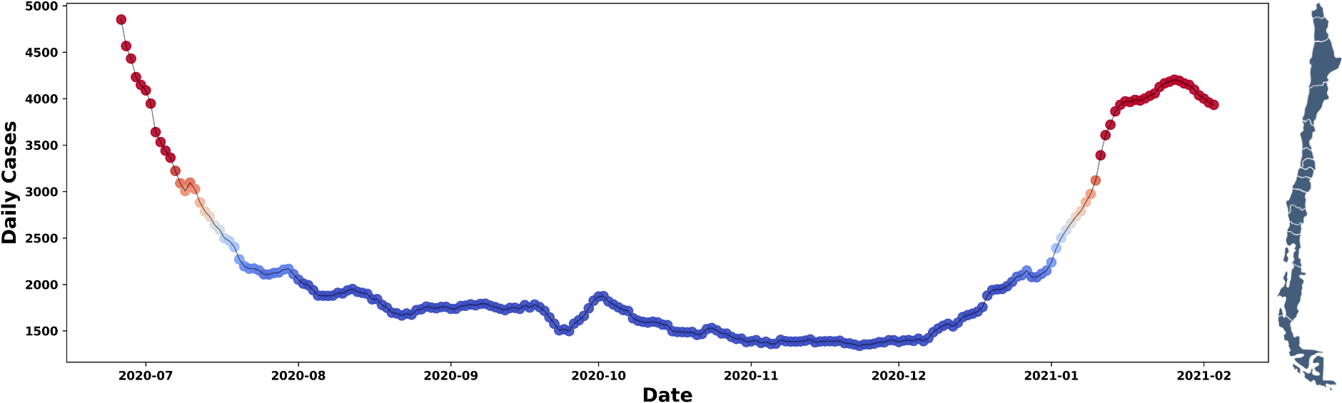
The colours indicate the magnitude: red (≥ 3000); orange (2501 to 2999); and in blue (≤ 2500) we highlight a prolonged trough with a minimum of 1338 cases on 23 November 2020.
WHO: World Health Organisation.
Source: compiled by the authors based on WHO records [4].

Full size

Indeed, traditional mathematical models, based on the classic SIR compartmental model and assuming a constant transmission rate, are inherently incapable of reproducing sequences of peaks and troughs. This is because they tend to predict unimodal incidence curves with sharp peaks [7,8,9]. As Chowell et al. point out, “simple epidemic growth models assume constant transmission rates and homogeneous mixing, which generally results in unimodal incidence curves that do not capture the complex resurgence patterns observed in historical pandemics” [10]. It is widely accepted that temporal variability in the transmission rate, driven by behavioural changes, public health interventions and population adherence to these, is fundamental to explaining such dynamics [11]. In turn, Flaxman et al. [12] demonstrated that non-pharmaceutical interventions, particularly lockdowns, significantly reduced transmission by substantially altering the effective reproduction number.

Broadly speaking, there are two strategic modeling approaches to incorporate this variability:

1. Imposing an explicit, a priori functional form for the transmission rate (for example, a function that decreases over time) [13,14,15,16].

2. Incorporating a dynamic law governing its evolution as a function of the system’s state variables [11,17].

Recently, the second approach has seen significant advances with the formulation of the mechanical theory of contagion [18,19,20]. An underlying objective of this article is to disseminate the language of the mechanical theory of contagion using a simple example represented by a basic model. Note that this theory provides a formal framework that allows the dynamics of the transmission rate to be derived from first principles, thereby avoiding ad hoc assumptions. These principles revolve around mechanisms of action and reaction associated with the loss and acquisition of intrinsic protective behaviours, linked to the implementation of pharmaceutical and non-pharmaceutical interventions [11,21,22]. Consequently, adherence to and compliance with these measures by the majority of the population influence the increase or decrease in the spread of the pathogen through social behaviour [23,24,25,26].

It is well documented that human behaviour is a key factor in fluctuations in the transmission rate [27,28,29]. The hypothesis put forward is that keeping the transmission rate below its natural or intrinsic level requires sustained behavioural effort on the part of the public. This led to a stabilisation which, in particular, allowed hospital demand to be kept generally below capacity, even taking into account capacity increases [30,31,32,33]. It should be noted that during this period, vaccines were not yet available [34].

In this context, our aim is to understand, from a general perspective, the behaviour of the infection rate in Chile during the period from July to December 2020, using the recent conceptual framework of the mechanical theory of contagion. We seek to quantify the collective effort required, in terms of reducing and stabilising the infection rate, to keep hospital demand at manageable levels. The results of the analysis not only validate the model’s explanatory power but also offer a mechanistic perspective on the population’s response to prolonged control measures in a critical scenario.

The article is structured into the following sections:

• Methods, where the theoretical framework of the β-SIR model is developed, formalising the incorporation of a variable transmission rate governed by mechanistic-behavioural principles.

• Results, in which a systematic numerical exploration is carried out to validate the model against data observed in Chile.

• Discussions and conclusions, where the findings are summarised and future research directions are outlined.

Methods

We will consider a population affected by the spread of an infectious disease that follows the basic SIR compartmental epidemiological model. That is, each individual can be classified as susceptible (S), infectious (I) or recovered (R), and a unidirectional flow S → I → R is described by the system

(1)S′(t)=−D(t),    I′(t)=D(t)−γI(t)   y    R′(t)=γI(t)

Where D(t) is the number of new cases, considering the time variable in days. Typically, the variable D(·) is expressed in accordance with the law of mass action, such that D(t) = β(t)S(t)I(t)/N, with N = S + I + R the population size (constant), β(·) the transmission rate and γ-1 the duration of the period of transmissibility.

Assuming that, in human populations, a threat to life triggers a defensive response in individuals (in a similar way to what occurs in ecological communities, where prey seek shelter in the presence or under direct threat of a predator [35]), it is possible to consider the existence of a population fraction f (0 ≤ f ≤ 1) whether it adheres to non-pharmaceutical mitigation measures or disregards them (stops seeking shelter). All of this is based on an assessment of the size of the active group . This suggests that if is too high, then f`∼ µmax(1 - f). Meaning, there exists a flow, less than or equal to µmax, through which the non-refuigiated is added to f. Conversely, if I is comparatively low, then f` ∼ -νmax f. This means that a maximum rate for the cessation of refugee status has been set.

Regarding µmax and νmax, which we shall refer to as the maximum protection factor and the maximum unprotected factor, respectively; note that both can be interpreted as upper bounds of their respective factors of the same name µ(I) and ν(I). These values reflect, over time, an assessment of the status of pathogen spread, for example through the number of active individuals I(t) in the t-day. Thus, taking into account the natural growth pattern for the protection factor µ(I) and a decreasing trend for the vulnerability factor ν(I), we opted for technical simplicity and chose the following expressions:

(2)μ(I)=μmaxII+Iu/2     and     ν(I)=νmaxIν/2I+Iν/2

Let’s observe in (2) that µ(·) is strictly increasing, reaching half its maximum in Iµ/2, while in ν(·) is strictly decreasing, reaching half its maximum value at Iν/2.

Thus, the change in the refugee population, estimated based on the balance between daily arrivals and departures, is given by

(3)f′=μ(I)(1−f)−ν(I)f,withf0:=f(0)≤1.

A key factor is understanding how this group of refugees affects the transmission rate β(·). To this end, the work by Melikechi O et al. [9] introduces the concept of an epi-bandVδ,τ (P), defined as the spatiotemporal region surrounding an individual P, which makes it possible to determine whether contact has occurred when a person has remained at a maximum distance δ during a minimum τ time . This allows the transmission rate to be expressed as the product κgen · ρ, where κgen, known as the general contact rate, represents the average number of times per day that any given individual Q enters Vδ,τ (P). The ρ parameter indicates, in turn, the probability that, given contact between Q and P, being P infectious and Q infected.

If we consider the fraction f to represent the proportion of the population that is in isolation, it is to be expected that, under this assumption and given the lack of opportunities for contact, the overall number of contacts within the non-isolated population, κgen*, reduces in proportion f, adopting (1-f)κgen the value. Therefore, assuming a constant transmission rate β* in the absence of insulation, we have

(4)β(t)=κgen(t)⋅ρ={(1−f(t))κgen∗}⋅ρ=(1−f(t)){κgen∗ρ}=(1−f(t))β∗

Therefore, by deriving the identity in (4), we obtain β` = -f`β*; and so, using (3), we have

(5)β′={μ(I)(1−f)−ν(I)f}β∗=ν(I)(β∗−β)−μ(I)β

This equation corresponds to the reaction–replenishment dynamic law governing the transmission rate that Córdova-Lepe and Vogt-Geisse [20] refer to µ(I)β(t). It represents the ‘reaction rate’, that is, the speed at which the population adopts protective behaviors. For its part, ν(I)(β* -β(t)) it corresponds to the ‘restoration rate’, the component that tends to bring the system back to the intrinsic rate β∗, by analogy with the processes of isolation and exposure in the presence of an infectious agent.

Therefore, highlighting the dynamic nature of β(·) in the system (1)-(5), we shall denominate β-SIR to the system:

(6){β′(t)=ν(I(t))(β∗−β(t))−μ(I(t))β(t),S′(t)=−β(t)S(t)I(t)N,I′(t)=β(t)S(t)I(t)N−γI(t),R′(t)=γI(t).

With initial status S(0), I(0) and R(0) so that S(0) + I(0) + R(0) = N, and ν(·) and µ(·) are given by the functional structures presented in (2).

Introducing the concept of the ‘intrinsic reproduction number’, denoted by R0* := β*/γ. Our study examines the case R0* §amp;gt; 1. This represents, at least initially, an epidemiological spread. Therefore, in model (6), an initial transmission rate 0 §amp;lt; β(0) ≤ β* is assumed. This reflects the existence of a level of public concern that causes the process to begin with a transmission rate that is lower than, or at most equal to, the intrinsic (natural) rate β*.

Within the framework of contagion dynamics, introduced by Córdova-Lepe [18], the Second Law of Contagion concerns the balance between the strength of contagion FI and forces of contact Fc, represented in our work in FI = (βI)` and Fc = I`β, so that

FI−Fc=(βI)′−I′β=β′I+βI′−I′β=β′I=ν(I)(β∗−β)I⏟Fext1−μ(I)βI⏟Fext2

where, denoted by [t] per unit of time (days) and by [ind] As for individuals, we see that two external forces are at work: one of protection Fext1 and the other of desprotection Fext2, defined by

Fext1=ν(I)[t]-1(β*-β(t))[t]-1I(t)[ind] and Fext2=μ(I)[t]-1β(t)[t]-1I(t)[ind].

Please note that we have highlighted the units [ind/t2] in line with the unit associated with the concepts of force introduced by Córdova-Lepe F [18].

Since our focus is on the transient behaviour of model (6) (a very specific initial period associated with 2020), an analysis of its long-term behaviour is not of interest to us. However, it should be noted that if β(0) ≤ β*, then β(·) ≤ β* always. Indeed, it is worth noting that, intuitively, mitigation measures and population responses can only reduce transmission below its natural level; they can never increase it above its intrinsic level. In fact, by defining the auxiliary function as u(t) = β* -β(t), we measure the deviation of the transmission rate from its intrinsic value. We calculate its derivative, and obtain: u`(t) = µ(I(t))β* - [ν(I(t)) + µ(I(t))]u(t). Note that this is a non-homogeneous linear differential equation for u(t). Let us consider the integral factor Φ(t) = exp(J(t)) §amp;gt; 0, with J(t) = ∫[0,t] [ν(I(s)) + µ(I(s))] ds, which is strictly positive for all t ≥ 0. Multiplying both sides of the equation by Φ(t) and integrating this expression over 0 and t, the clearance is made:

u(t)={u(0)+β*∫0tΦ(s)μ(I(s))ds}/Φ(t).

Therefore, we observe that u(0) = β* - β(0) ≥ 0, by hypothesis, we obtain u(t) ≥ 0 for every t ≥ 0. Equivalently, we have β(t) ≤ β* for every t ≥ 0.

This finding has significant epidemiological implications. The effective transmission rate never exceeds the intrinsic rate β*. This confirms that social distancing and mitigation measures can only suppress transmission below its natural level; they can never increase it. This property ensures that the model adheres to a fundamental epidemiological threshold and provides a natural constraint on the system’s dynamics.

Results

Depending on different estimated values of the intrinsic reproduction number R0*, As reported by Navas & Vergara-Hermosilla [15], Tariq et al [36] and Canals et al [35], we analysed three epidemiological scenarios by fitting the model (1)–(5). To this end, the parameters were determined νmax, μmax, Iν/2and Iµ/2, which define the dynamic law governing the reaction–recovery transmission rate (5). These parameters were estimated using the non-linear least squares method, implemented in Python via the function scipy.optimize.leastsquares. His routine is available via the following link: Google-Colaboratory

The initial conditions were derived from data reported by the Chilean Ministry of Health in its 10 July 2020 report [3]. In particular, the following were taken into account: I(0)= 26 390 active cases R(0)= 284 834 removed cases, that is, those who have recovered or died; together with a Chilean population of N = 19,660,000 individuals. Consequently, the number of susceptible individuals was calculated using the identity S(0) = N -(I(0)+R(0)), with a total of S(0)= 19 348 776 individuals.

Scenario 1

Taking into account an average incubation period of γ-1 = 7 days for an infectious individual, and an intrinsic transmission rate β* calculated on the basis of the intrinsic basic reproduction number given by β*=R0*γ, by R0*=1.8 as reported by Navas and Vergara-Hermosilla [15], the following is obtained β* = 0.257. The adjustment for new cases is illustrated in Figure 2.

Figure 2

Trend in new and estimated COVID-19 cases, scenario 1.

Data (black dots) and fit (blue line), based on model (6), showing the trend in COVID-19 cases in Chile from July to December 2020.
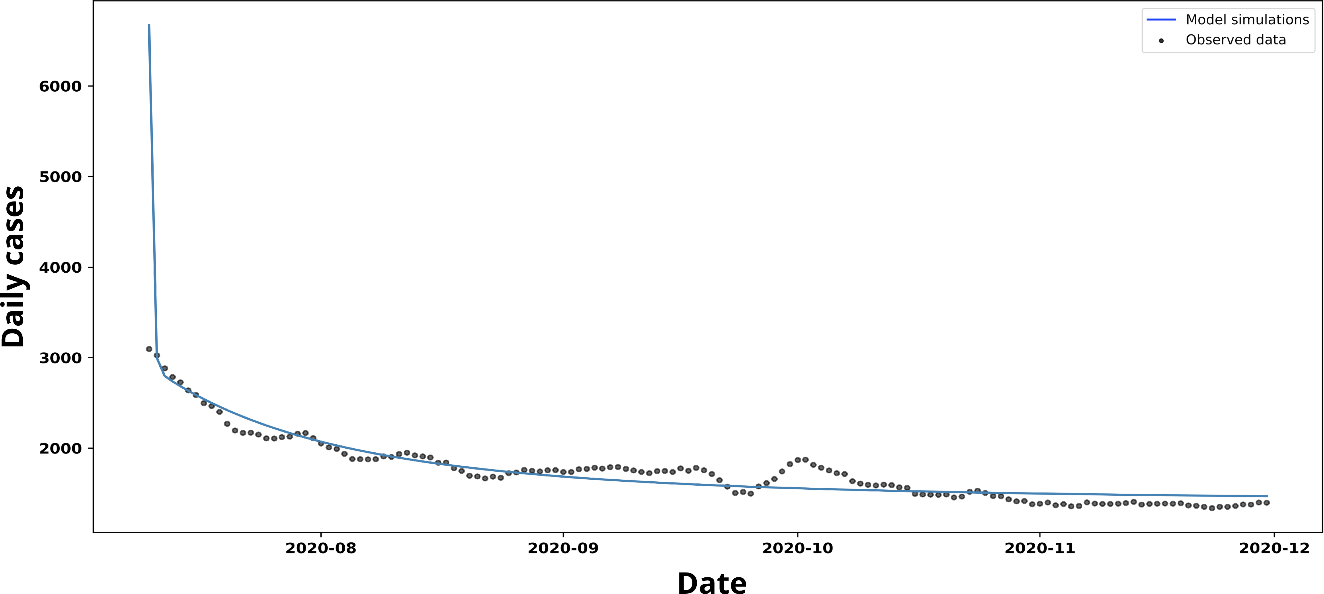
Source: Prepared by the authors based on the study’s results.

Full size

The fit based on the non-linear least squares method yielded the following values µmax = 1.55 and Iµ/2 = 10, which means that the protection factor meets µ(I)≈ µmax. This is because the number of infectious people, I(t), remains well above the threshold Iµ/2 (Figure 3).

Figure 3

Parameter tuning, scenario 1.

In (a), simulation of the protection factors µ(I(t)).
In (b), corresponding behaviour of the dynamic transmission loop tβ(t).
Source: Prepared by the authors based on the study results.

Full size

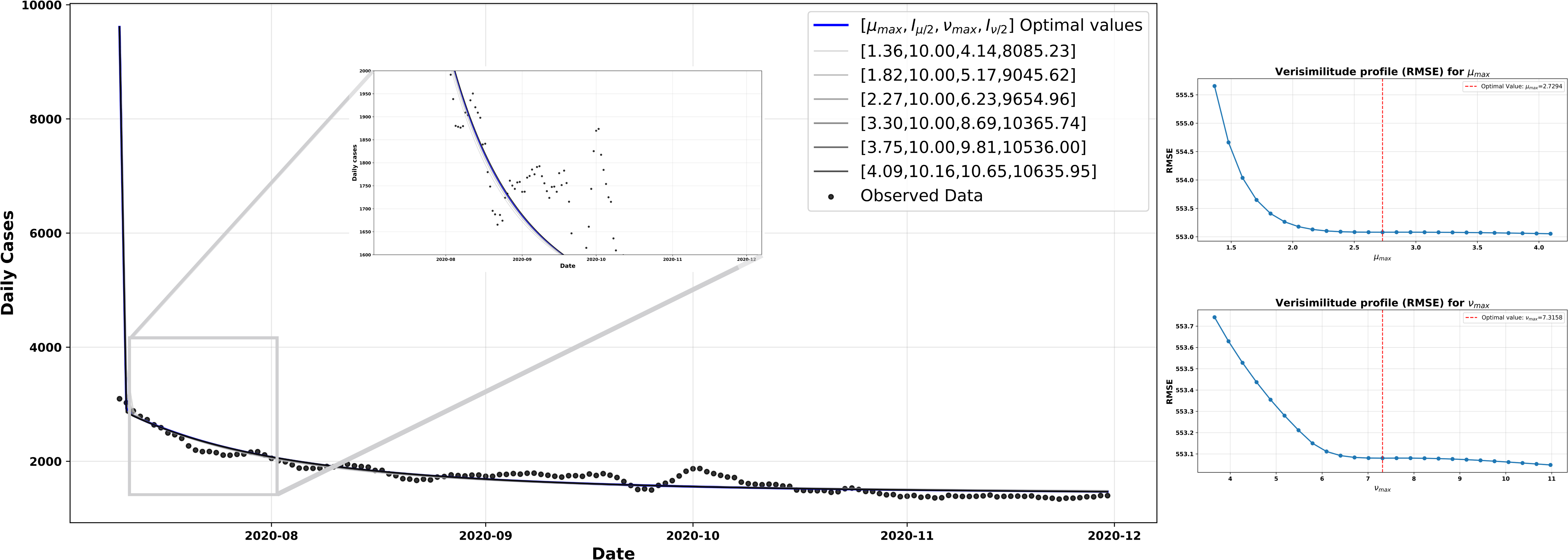
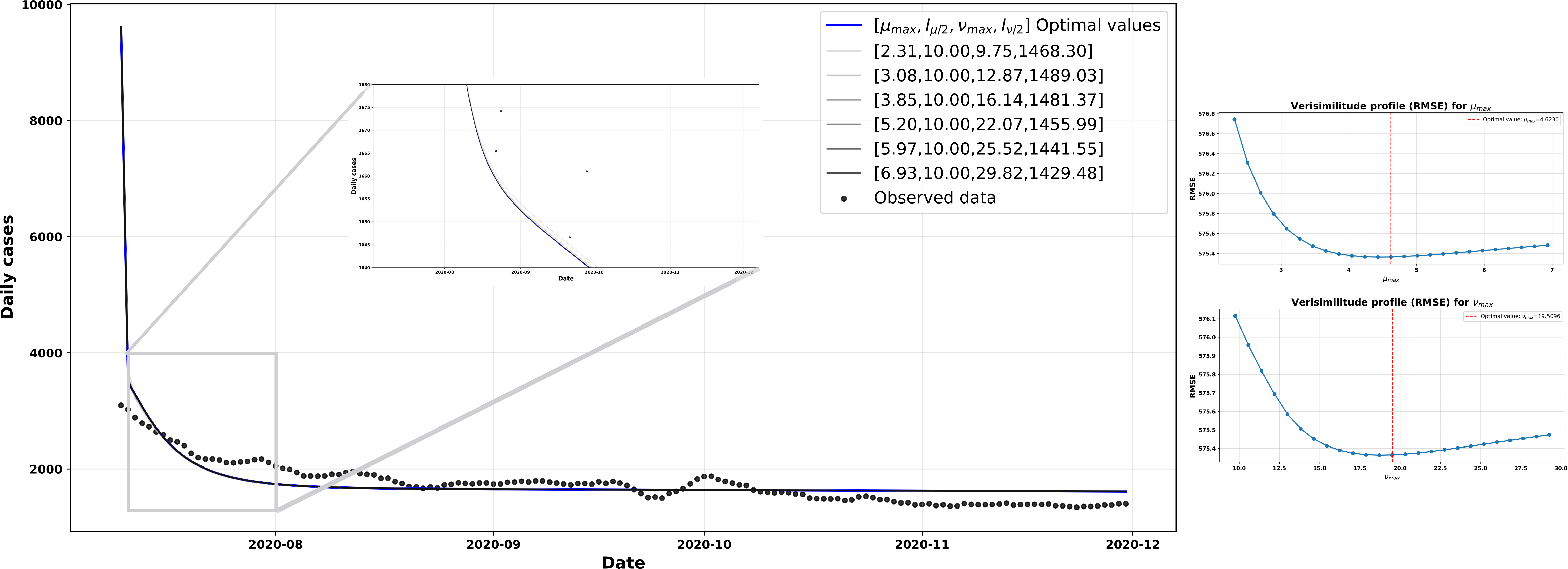
In Figure 3, β(t)shows a marked decline, influenced by the protective factor (µ(I)≈ µmax) and low unprotected value (ν(I)) at the start of the study. Subsequently, this transmission rate rises in line with the gradual increase in the vulnerability factor ν(I).

However, these adjusted values for protection and unprotection are difficult to identify in practice. As shown in the root mean square error (RMSE) curves in Figure 4, although both parameters can be estimated within the explored range, neither exhibits a clearly defined minimum. Rather than converging towards a clearly marked optimal value, the curves gradually flatten out and appear to settle at a local minimum.

Figure 4

Adjustment of protection and de-protection parameters, scenario 1.

The left-hand side shows model simulations obtained by shifting the optimal values of the parameters µmax and Vmax’ by 50%, compared with the observed data. On the right are the likelihood profiles based on the RMSE for µmax (top) and Vmax’ (bottom), where the red vertical line indicates the estimated optimal value for each parameter.
RMSE: root mean square error.
Source: Prepared by the authors based on the study results.

Full size

This behaviour is consistent with what occurs during model fitting in this scenario: the parameters do not act independently. The epidemiological dynamics are non-linear and coupled, such that a change in any of the parameters alters the course of S(t), I(t) and R(t). To compensate for these variations, the adjustment redistributes the values of the other parameters, generating different combinations of [νmax, Iν/2, μmax, Iμ/2] which produce simulated trajectories that are virtually indistinguishable. As a result of this internal compensation, the model can reproduce the data accurately across multiple parameter configurations. This makes it difficult to identify a single set of optimal values with precision.

The multiple configurations used for the simulations in Figure 4 were explored in a controlled manner by applying ±50% variations to the parameters νmax and μmax obtained using the least squares method. We observe that the changes in the shape of the simulated curves are relatively small, whilst the root mean square error shows much more pronounced variations. This means that, even when we make significant changes νmax and μmax and we re-optimise the remaining parameters, the overall dynamics of S(t), I(t)and R(t) remains virtually unchanged. This behaviour indicates that the model is not very sensitive in dynamic terms, but highly sensitive in terms of fit. This reinforces the idea that it allows multiple parameter combinations to generate similar trajectories.

Scenario 2

For the simulation of scenario two, shown in Figure 5, an initial transmission rate was implemented β0 = 0.37, an intrinsic transmission rate β* = 0,81 and a removal rate γ = 0,426 calculated by a relation γ = β*/R0, with a basic reproductive value R0 = 1.9. These values were derived from the generalised growth model described by Tariq et al. in [36].

Figure 5

Trend in new and estimated COVID-19 cases, scenario 2.

Comparative graph showing the trend in new COVID-19 cases in Chile and the trend in new cases estimated by our β-SIR model, as given by equation (6).
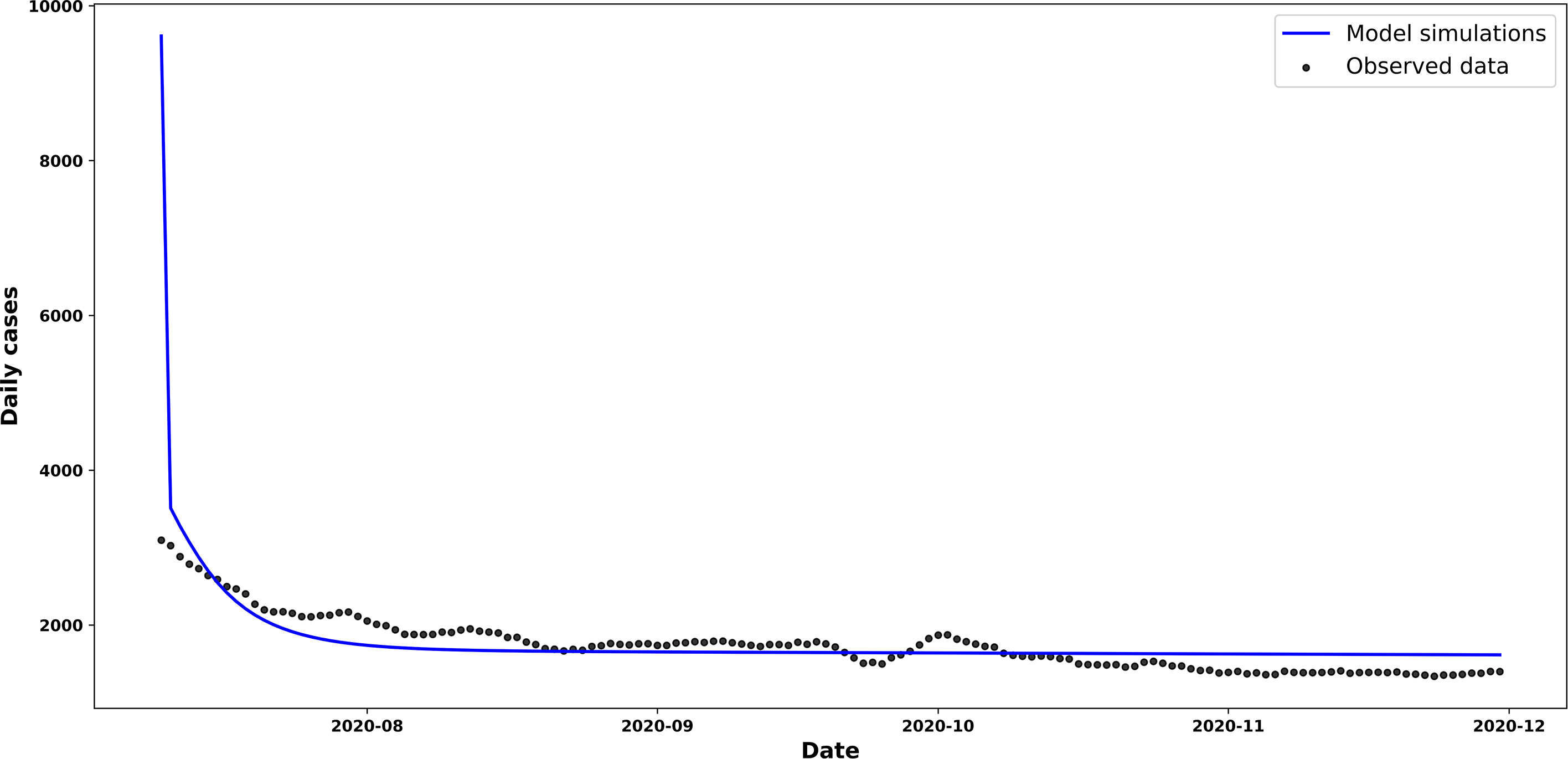
Source: prepared by the authors based on the study’s results.

Full size

The curve of new cases shown in Figure 5 follows a trend very similar to that simulated using the parameters of Scenario 1. However, the model slightly overestimates the number of cases towards the end of the period, whilst fitting the data quite accurately from the first few weeks onwards.

The non-linear least squares fit shown in Figure 6 yielded the values for the protection and unprotection parametersµmax = 4.62, Iµ/2 = 10, νmax=19.5 and Iν/2=1467. A comparison between the model simulations under different scenarios (Figures 4 and 6) and the observed data shows that, even with small variations in transmission rates, the simulated curves maintain a generally stable shape, accurately capturing the downward trend and plateau in the observed daily case numbers. This suggests that the model exhibits structural robustness, in the sense that its qualitative behaviour is not significantly affected by moderate changes in the parameters of the transmission mechanism. In other words, although the numerical values of β0, β* or even if the protective factors vary within a reasonable range, the simulated dynamics continue to consistently reproduce the observed trend in cases. This indicates that the system is stable in the face of moderate parametric perturbations, and that its qualitative conclusions do not depend critically on a single, precise set of parameters.

Figure 6

Adjustment of protection and de-protection parameters, scenario 2.

The left-hand side shows model simulations obtained by shifting the optimal values of the parameters µmax and Vmax’ by 50%, compared with the observed data. On the right are the likelihood profiles based on the RMSE for µmax (top) and Vmax’ (bottom), where the red vertical line indicates the estimated optimal value for each parameter.
RMSE: root mean square error.
Source: Prepared by the authors based on the study results.

Full size

Scenario 3

In this scenario, we present the simulations based on the rates used and estimated by Canals et al [20]. In this study, the size of the Chilean population was taken as N = 19 000 000, and the period during which an individual remains infectious or dies was set at 14 days, then γ = 1/14 and a basic reproduction number in mid-June of less than 1, thus resulting in β(0) = 0.0714. Furthermore, an average intrinsic basic reproduction number of β* = R0γ= 1.516, on the basis of which the intrinsic transmission rate was calculated β*= 0.1082, under β* = R0γ ratio.

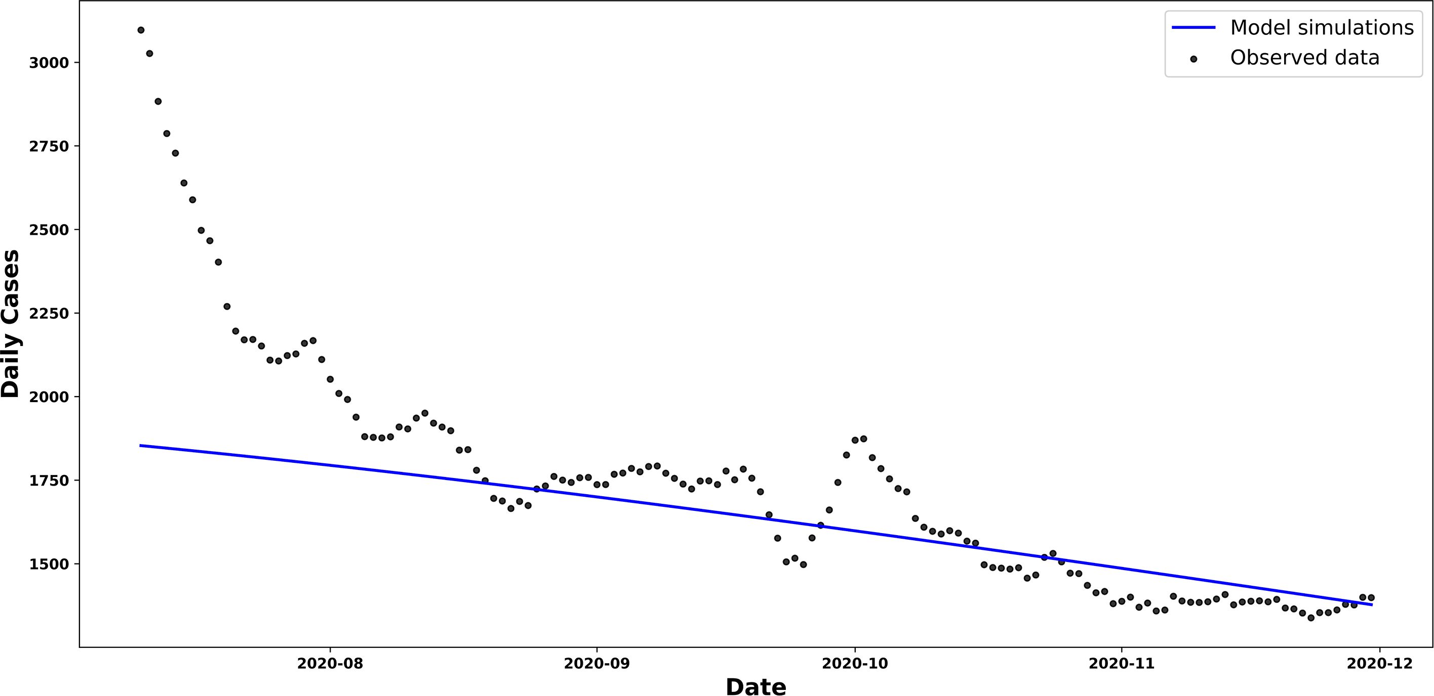
The curve of new cases shown in Figure 7 exhibits a linear trend that differs significantly from the simulated curves in the previous scenarios. It can be seen that the β-SIR model (6) underestimates the initial number of new cases, but begins to align with the data by mid-August. This is likely due to the low initial transmission rate reported in mid-June [35], which may differ in July, the period covered by this study.

Figure 7

Trend in new and estimated COVID-19 cases, scenario 3.

Comparative graph showing the trend in new COVID-19 cases in Chile and the trend in new cases estimated by our β-SIR model, as given by equation (6).

Source: prepared by the authors based on the study’s results.

Full size

The protection parameters set for this scenario were µmax= 1.06 × 10-4, Iµ/2= 10. We obtain µ(I) ≈ µmax, given that the number of active cases remains very high compared with the threshold value I/2.

As for the adjusted vulnerability parameters, they were νmax= 1 × 10^-4 and β* = R0γ 1 000 000. This indicates that the vulnerability factor ν(I) ≈ νmax, This occurs in this case because the threshold takes precedence Iν/2 on confirmed cases I(t).

Consequently, the protective effect provided by µ(I) is essentially active at its maximum level, just like the unprotected factor ν(I). However, ν(I)contributes less to the momentum because it is lower than µ(I). This combination explains the slight decline observed in the transmission rate β(t) and active cases I(t) in Figure 3.

The various configurations used for the simulations in Figure 8 were explored by applying ±50% variations to the parameters νmax and μmax obtained using the least squares method. We note that the changes in the shape of the simulated curves are again small, whilst the root mean square error = 272 is lower than in the previous scenarios.

Figure 8

. Adjustment of protection and de-protection parameters, scenario 3.

The left-hand side shows model simulations obtained by shifting the optimal values of the parameters µmax and Vmax’ by 50%, compared with the observed data. On the right are the likelihood profiles based on the RMSE for µmax (top) and Vmax’ (bottom), where the red vertical line indicates the estimated optimal value for each parameter.

RMSE: root mean square error.
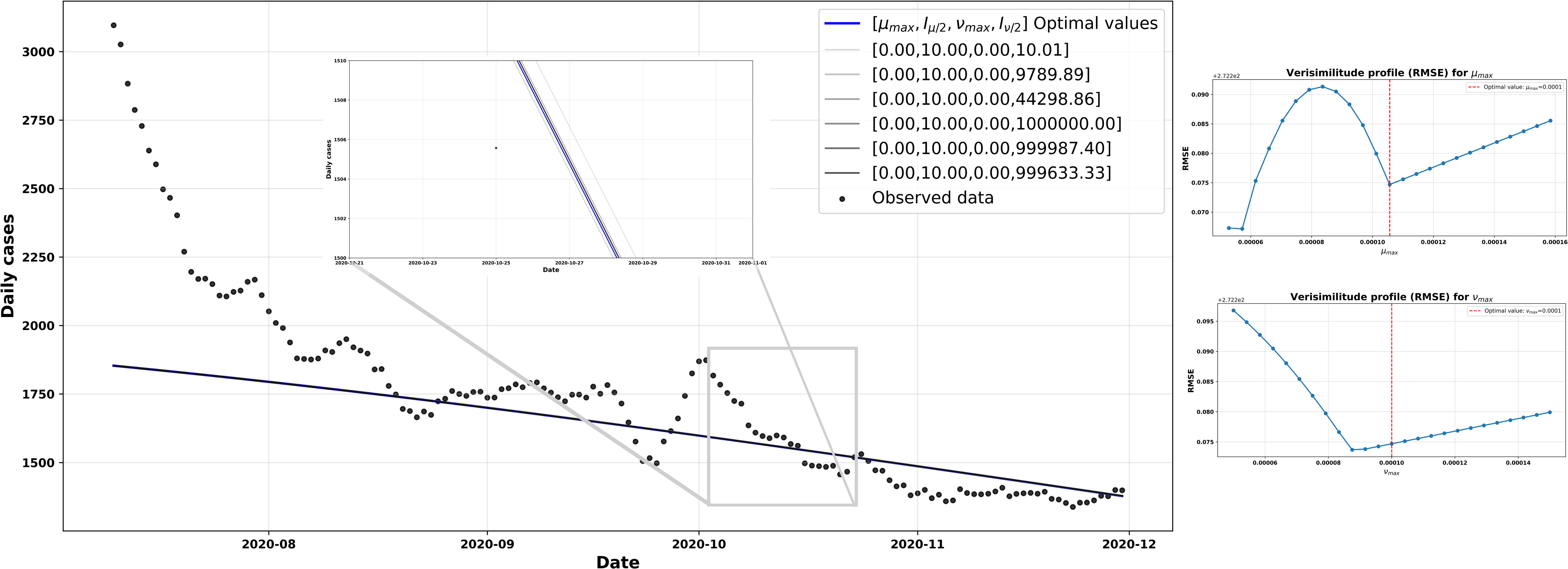
Source: Prepared by the authors of this study.

Full size

Scenario 4

In this final scenario, we expanded our analysis by explicitly incorporating the effect of the non-pharmaceutical measures implemented in Chile on the model’s dynamics. To do this, we used the composite stringency index. This indicator combines nine types of government interventions, including school and workplace closures, movement restrictions, and travel bans. This index ranges from 0 to 100, with higher values representing stricter policies, as reported by the World Health Organisation (WHO) [4].

The central idea was to allow the maximum protection parameter, μmax , to respond directly to the temporal variation in this index. To this end, a simple proportional relationship was used:

μmax*=μmax∙stringency indexaverage stringency index ,

where the average stringency index was calculated over the period from 26 June 2020 to 30 January 2021, corresponding to the extended interval used in the simulation. Under this formulation, when the country adopts stricter measures, the protective effect incorporated into the model increases. Conversely, when measures are relaxed, this effect decreases. With this formulation, the initial conditions and parameters were selected μmax, Iμ/2, νmax, Iν/2 optimised arbitrarily from scenario 1. Figure 9 shows the simulated behaviour compared with the observed data, reflecting the model’s response to variations in the severity index over μmax.

Figure 9

Rigor index.

Variation in the rigor index with respect to µmax.

Source: compiled by the authors based on the study’s results.

Full size

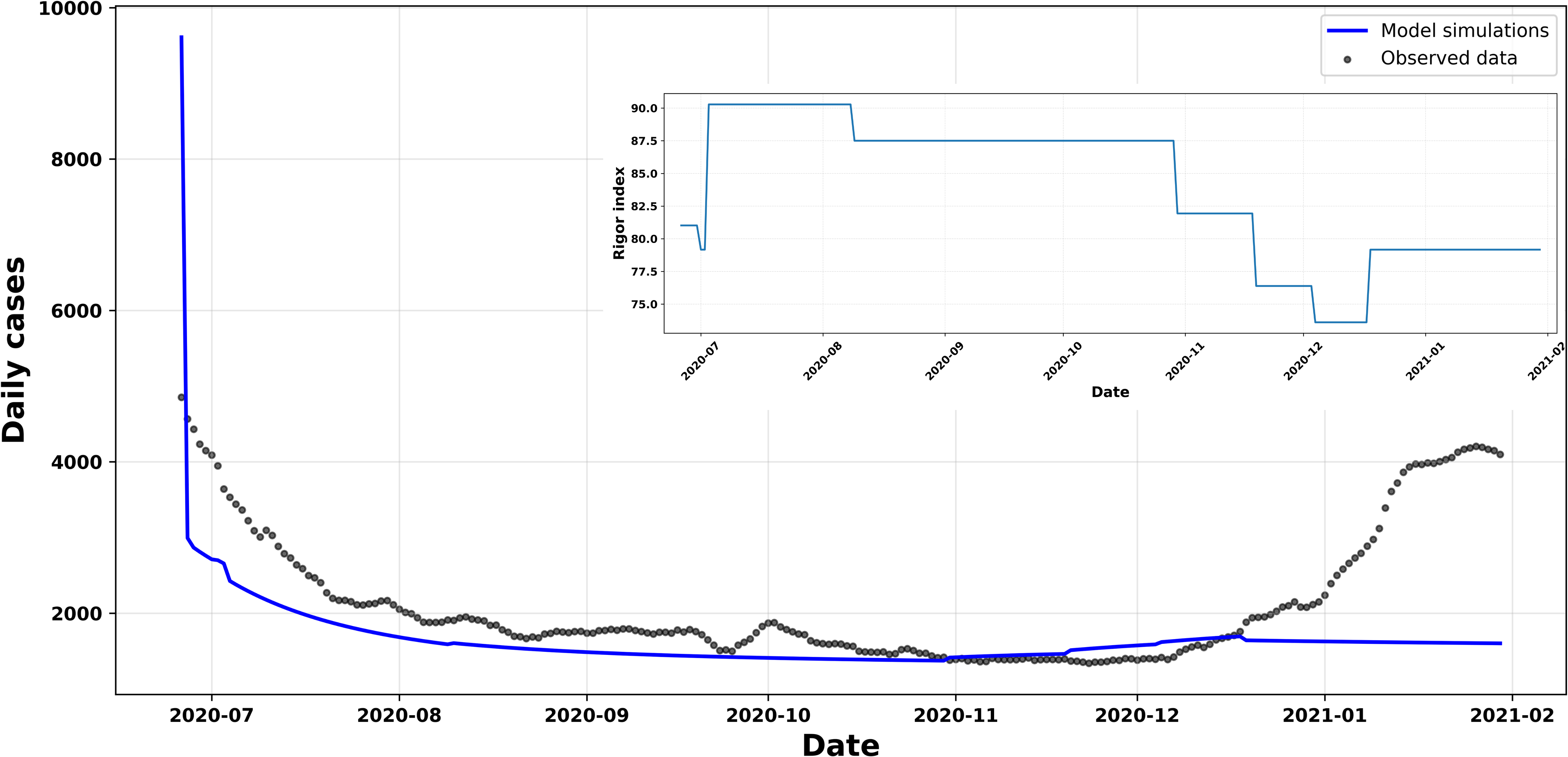
By incorporating the composite severity index into Figure 9, we observe that the parameters associated with the protection mechanism, in particular μmax, vary in ways consistent with daily changes in the intensity of non-pharmaceutical measures. On days when measures are most stringent (for example, values close to 90), the model’s simulation of new cases decreases, suggesting a greater ability of the population to enter a state of protection. Conversely, when the index decreases slightly (as occurs around 1 July), the maximum protection factor also decreases, reflecting lower protective pressure. Throughout the analysed period, this relationship remains stable and does not generate abrupt fluctuations in the parameters, indicating that the model responds consistently and robustly to moderate changes in stringency.

Taken together, these results show that the model is capable of adequately capturing the influence of public policies on the population’s protective behaviour, whilst maintaining structural stability in its parameters throughout the adjustment.

Finally, we can observe in Table 1 that the model β-SIR As shown in (6), this provides a very good description of the trough in daily new COVID-19 cases during the period from July to December 2020. This suggests that the equations proposed for the protective and non-protective factors are appropriate.

Furthermore, the protective parameters applied to the transmission rate β—which were estimated using the non-linear least squares method within this model—enable us to determine, starting from the threshold of active cases (Iµ/2), the extent to which non-pharmacological intervention policies and government-imposed mobility restrictions affect the Chilean population. Similarly, the µmax estimate characterises the speed with which these mitigation measures are adopted.

The data suggest that these measures did not significantly impact the eradication of the disease. Chambon et al. [37] argue that the expected trajectory of the outbreak is influenced by the ‘unengaged’ or ‘non-compliant’ population in relation to non-pharmaceutical measures. Furthermore, they note that adherence to mitigation measures declines over time; and that factors such as pandemic fatigue, a perceived decrease in risk, and the normalisation of social contact limit the effectiveness of interventions.

The threshold value Iν/2 implemented in the transmission rate β, fitted using the non-linear least squares method under this model, allows us to determine the number of active cases at which the ‘unengaged’ or ‘non-compliant’ population begins to decline and accept the mitigation measures. Furthermore, the value of νmax allowed us to see the rate at which people adopt this type of disobedient behaviour.

Note that a common feature across all scenarios is the stabilisation of daily cases, a situation that persists as long as the external protective force Fext2 and its inverse Fext1 remain in effect. Therefore, as regards maintaining the model beyond December, this is not possible as complexities arise, such as variants, vaccination and various behavioural factors linked to the end-of-year festivities, the summer holidays or expectations regarding vaccination itself. These aspects mean that a model ceases to be a baseline model; it must incorporate additional compartments and account for varying intensity parameters. In this regard, to reproduce the January 2021 data (shown in orange or red in Figure 1), we vary the model parameters and obtain Figure 9.

Discussion and conclusions

When faced with an epidemic curve, determining what constitutes a wave is not a settled matter, as there is no universal objective definition. This lack of consensus has direct consequences for detailed data analysis [38]. In this study, for the COVID-19 data in Chile during 2020, we have selected a period falling between the first two so-called waves. In a population of nearly twenty million people, the daily case curve shows relative stability which, at first glance (see Figure 1), forms a flat or trough-like section. We refer to what is commonly termed a trough, roughly bounded between early July (following a peak of 6,938 cases on 14 June [39]) and late December (prior to a new peak on 9 January 2021, with 4,956 cases). This period, associated with the dominant ‘Delta’ variant [40], shows a well-defined trough with a low of 1,352 cases on 22 November. This is of great interest for understanding the causes of this dynamic pattern of controlled or reduced transmission.

The literature suggests that these troughs may be due to a combination of factors, notably the depletion of susceptible individuals, seasonal changes, the effectiveness of control measures, and population behaviour. Ruling out the first two causes, we understand that, in the Chilean case, the observed stability is mainly associated with the implementation of health restrictions and a sufficiently alert population, willing to maintain, albeit to a decreasing extent, preventive behaviours. In this regard, the model with β(·) the dynamic described in Equation (6), and illustrated in Figure 2, is consistent with this interpretation. It is worth noting that similar periods of stability, in the form of troughs or plateaus, were observed in numerous countries, which reinforces the importance of the mitigation efforts undertaken by the respective health authorities [41].

It is possible to speculate that this trough began to disappear around January 2021, when figures rose again, probably due to behavioural factors associated with the end-of-year festivities, the start of the summer season and the announcement (on 16 December) of the arrival of 20,000 vaccine doses. This announcement materialised on the 24th of the same month, with the first person being vaccinated in the country [42].

The knowledge generated for decision-makers, most of whom belong to the medical community and the political sphere, is indispensable in the management of a high-risk infectious pandemic. For their part, mathematical models, given the phenomenon’s complexity, constitute essential tools. Hence the need to strengthen educational efforts in this direction, in order to better understand the course of transmission processes [43].

The aim of this article has been to present a structurally simple mathematical model—for example, one with a small number of compartments—yet capable of providing a description that is reasonably consistent with the data. Undoubtedly, even simple models play a significant role in the monitoring of epidemics, as they help to rationalise decision-making by tracking the dynamics without losing explanatory power [44]. In particular, this approach allows for an interpretative reading grounded in the language of the mechanics of infection, which introduces a Newtonian analogy based on concepts of force. From this perspective, non-pharmaceutical mitigation measures can be understood as a reaction force exerted by the population, the counterpart to the intrinsic cultural and environmental pressure driving a return to a natural state. However, the model is not viable for projections beyond the time interval considered. Indeed, after December 2020, it is no longer possible to assume that the system governing the dynamics remains a basic SIR model, as this assumption is unsustainable. This is because one must take into account the emergence of variants (non-homogeneous virulence and latency) and new structures arising from the multiplication of population compartments (for example, new infectious types), or the reduction in the susceptible population due to vaccination.

It should be noted that the usefulness or limitations of the mechanics of transmission—a theory which, in this paper, has been presented primarily as a descriptive and interpretative tool within a simplified empirical and theoretical context—depend on the modeler’s ability to transpose, by analogy, the physics of classical mechanics of multi-component systems into the language of transmission forces offered by the theory. An example of this application is in more complex epidemiological scenarios, such as the forces acting on transmission rates differentiated according to some compartmentalisation criterion (such as infectious types). However, for a more direct and comprehensive understanding of the scope and limits of the mechanics of contagion, the reader is invited to delve into the seminal publications [11,19,20] and the dynamics of the novel theory [18].