Introduction

In the healthcare setting, professionals must make decisions in a context of uncertainty. In making a diagnosis, clinicians categorize patient experiences into a particular condition that involves specific pathogenesis, treatment, and prognosis[1]. However, in most cases there is no absolute certainty whether a patient has the diagnosed condition or not[2].

More than a century ago, diagnostics were based on anamnesis and physical examination. According to Erick Cobo and colleagues, the English monk Thomas Bayes concluded that God’s existence could only be demonstrated if one first believed in God. Therefore, the probability that God exists depends on being a believer or not[3]. This reasoning applied to medical diagnosis states that the event probability after applying a test depends on the event probability prior to the test application, in addition to test characteristics[4]. The presumed probability prior to its test application is a process in which the health professional uses knowledge, experience, and clinical judgment[5].

In turn, there are other diagnostic approaches such as heuristics, defined by Perez[6] as “psychological mechanisms based on human performance in problem-solving, by which we reduce the uncertainty produced by our limitation in dealing with the complexity of environmental stimuli”. Thus, it is a fast and intuitive way of thinking that provides probability estimates for decision-making. However, the use of heuristics carries potential avoidable errors that can lead to incorrect diagnoses[7] (Example 1). Evidence-based medicine provides tools to “objectify” clinical experience, avoid biases, and facilitate the interpretation of clinical scenarios.

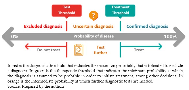
The information provided by diagnostic methods increases or decreases the probability of a particular condition[8], moving in between the diagnostic threshold and the therapeutic threshold (Figure 1). The diagnostic threshold reflects the minimum probability needed to consider a particular condition plausible, whereas the therapeutic threshold reflects the confidence needed in the diagnosis to initiate treatment. Below the diagnostic threshold, testing is not worthwhile because the diagnostic probability is low[2],[9]. Conversely, above the therapeutic threshold, the diagnosis has such a high probability that it justifies therapeutic decisions[2]. In between, when the diagnostic probability is intermediate, further testing is required to achieve a probability that is below the diagnostic threshold or above the treatment threshold[2],[9].

Figure 1.

Illustration of diagnostic and therapeutic thresholds.

Full size

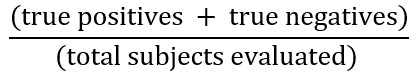
Diagnostic tests are a group of actions (including questions) to assess a patient’s history, signs on physical examination, and complementary tests (laboratory, procedural, or imaging) to determine the presence or absence of a condition. In some cases, they are also used to establish its severity. Diagnostic tests are evaluated for accuracy and impact. Accuracy is defined as the probability that the test result correctly predicts the existence and absence of a particular condition. This can also be interpreted as the relative frequency of subjects in whom the test got the diagnosis right, represented by the following formula:

However, it is important to consider that a diagnostic test can be more accurate in identifying sick patients or identifying healthy individuals; therefore, it may be helpful or not depending on the specific scenario[9].

Also, the accuracy of diagnostic tests can be represented by indicators such as sensitivity, specificity, positive predictive value, negative predictive value, likelihood ratios, and receiver operating characteristic (ROC) curves. These indicators are usually familiar to most general practitioners. However, there is evidence that they can be misapplied[10].

Accuracy assessment is performed by comparing the results obtained from the diagnostic test evaluated with a reference standard in the same group of patients. The reference standard –  also called gold standard – corresponds to a single test or combination of methods (composite gold standard), which allows establishing the presence or absence of a given condition[9]. For example, to diagnose acute pulmonary thromboembolism, the gold standard is computed tomography angiography. If the D-dimer latex agglutination test were used to diagnose the same condition, the estimation of the sensitivity and specificity of the results would be from the comparison of these with the gold standard[11]. The impact of a diagnostic test refers to how much a given diagnostic test result impacts patient care[12]. Therefore, impact assessment determines how the information provided by the test result affects therapeutic decisions and clinical outcomes[13].

A prospective short- and long-term follow-up study should be performed to determine the impact of a diagnostic test. Another alternative is to perform a retrospective study that allows monitoring, among other things, the number of diagnostic tests applied and the time delay until a definitive diagnosis or a definitive treatment. As a practical illustration, a cerebral vascular accident, without therapeutic alternatives (surgical or endovascular) because cerebral images indicate a poor prognosis, knowing lesions characteristics through new diagnostic tests would not affect the patient’s management[14].

This article is the seventh in a methodological series of thirteen narrative reviews on general topics in biostatistics and clinical epidemiology. This review explores and summarizes in a user-friendly language published articles available in the main databases and specialized reference texts. The series is oriented to the training of undergraduate and graduate students. It is carried out by the Chair of Evidence-Based Medicine of the School of Medicine of the Valparaíso University, Chile, in collaboration with the University Institute of the Italian Hospital of Buenos Aires, Argentina, and the UC Evidence Center of the Pontifical Catholic University of Chile. This manuscript aims to address the main theoretical and practical concepts of diagnostic testing in humans.

Probabilities and more probabilities in clinical reasoning

Probabilistic approaches are constantly used in medical practice to determine the probability that an individual has of suffering from a particular condition. This procedure is prior to performing a diagnostic test. This initial diagnostic approximation corresponds to the pre-test probability. This test depends on the clinician’s subjective assessment of the presence or absence of semiology findings to diagnose a particular condition of interest[15],[16]. In simplified form, it means that in the absence of additional relevant information, it has been accepted to use the condition’s prevalence under study to estimate the pre-test probability[15].

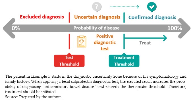
A negative diagnostic test with a high clinical suspicion or high pre-test probability (Example 3), or a positive diagnostic test with a low pre-test probability (Example 4), will make us doubt the test result in the first instance. When the pre-test probability is intermediate, the diagnostic test result may modify the uncertain probabilistic scenario to rule out or confirm the diagnostic suspicion (Example 5).

Problems with testing in the absence of uncertainty

Tests in the area of uncertainty

Figure 2.

Change in clinical behavior after applying a diagnostic test.

Full size

How do we measure diagnostic accuracy?

Sensitivity and specificity

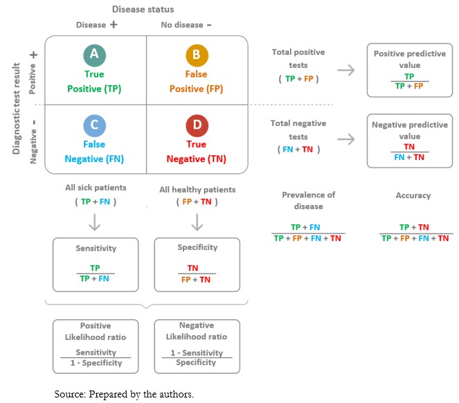
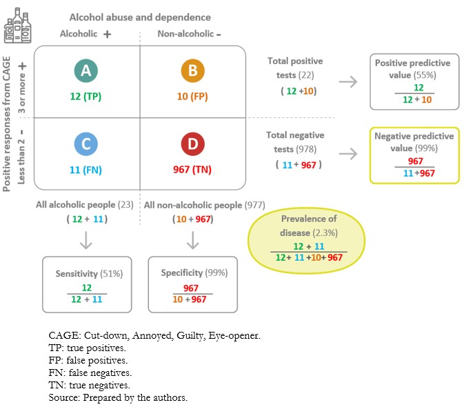
When applying a diagnostic test, there is the possibility of incorrectly classifying individuals who have undergone the test. Examples are alleged sick people who are healthy (false positives) and alleged healthy people who are sick (false negatives). The information on the values obtained for the test, in contrast to the values of the reference test or gold standard, is presented in tabular format (Figure 3). The so-called “2x2 contingency tables” are constructed with two columns. According to the reference standard, the columns correspond to the positive (left) and negative (right) result of the condition. To these are added two rows reflecting the positive (top) or the negative (bottom) result of the condition, according to the index test. In addition, a letter is designated to each cell[9]:

A. True positives: those sick individuals with a positive test result.
B. False positives: those healthy individuals with a positive test result.
C. False negatives: those sick individuals with a negative test result.
D. True negatives: those healthy individuals with a negative test result.

Figure 3.

Contingency table for the estimation of diagnostic accuracy.

Full size

Sensitivity” and “specificity”[2] are used to evaluate diagnostic tests. These are established values obtained from the diagnostic test application in a specific population at the validation time. In this sense, sensitivity and specificity are intrinsic properties of the diagnostic test. However, its performance also depends on the population characteristics in which it will be applied. These aspects are discussed in more detail later in the text[18].

Sensitivity is the probability that the test will correctly classify sick individuals or the probability that the sick individual will be positive[2]. Tests with high sensitivity are useful for screening because they have very few false negatives[19]. However, specificity is also important to avoid an excess of false positives, especially if these involve expensive or invasive confirmatory tests. In addition, because of the low number of false negatives, they are especially useful where failure to diagnose a specific disease or event may be dangerous or fatal to patients[16],[18].

Specificity is the probability that the test will correctly classify healthy individuals or the probability that healthy individuals will have a negative result[2]. A highly specific test has a very low false positive rate. Therefore, it has a high ability to confirm the disease. This means that if a highly specific test result is positive, there is a high chance of a true positive[18]. In clinical practice, tests with high specificity are preferred in confirming a diagnosis because of their low number of false positives. This is particularly important in severe diseases because timely mannered treatment can significantly reduce the physical, economic, and psychological consequences[16].

The estimation of the sensitivity and specificity of a diagnostic test will have greater applicability the broader the demographic and/or clinical characteristics of the sample of sick and healthy individuals in the population where the test will be used. Suppose the sample is representative of a population and the estimates are used in another population with different characteristics. In that case, the sensitivity and specificity values are incorrect, or at least not applicable to the population where the test is being used.

Since it is required to know patients’ health/sick status to calculate the sensitivity and specificity, it is necessary to contrast the diagnosis using a method that proposes an ideal parameter or gold standard (reference standard). This is the diagnostic technique that defines the presence of the condition with the highest known certainty[9],[19]. On the other hand, in routine clinical practice, health professionals are confronted with patients who consult them with the result of a test they have already undergone. The probability of being ill from the test results is known as predictive value. This topic will be developed below.

Positive and negative predictive values

A diagnostic test carries a certain probability that the result correctly categorizes the presence or absence of a disease; this corresponds to predictive values[20]. The positive predictive value is the probability that the diagnostic test correctly identifies sick individuals when it delivers a positive result. In turn, the negative predictive value is the probability that the diagnostic test correctly identifies healthy individuals when it delivers a negative result[21]. Ratios are used to calculate them (Figure 3).

Predictive values are conditioned by the a priori probability of the condition under study[18]. When the a priori probability is low, negative predictive values will be high, and positive predictive values will be low. In this scenario, a negative result of a diagnostic test with a high negative predictive value gives a higher probability to correctly rule out the patient’s condition than a positive result to confirm it. On the other hand, when the a priori probability is high, the positive predictive values will be high and the negative predictive values will be low. A positive diagnostic test result with a high positive predictive value gives a higher probability to confirm the condition than a negative result to rule it out[2],[16] (Examples 9A and 9B).

Figure 4.

Contingency table for locality “A”.

Full size

Figure 5.

Contingency table for location “B”.

Full size

Predictive values determine the post-test probability based on the diagnostic test result. However, predictive values are only comparable in populations with a similar prevalence or similar pre-test probability of the condition under study[19].

Likelihood ratios

Likelihood ratios compare the probability of finding a given result (positive or negative) of a diagnostic test in sick individuals in relation to the probability of finding that same result in healthy individuals[16]. Odds ratios are calculated using the sensitivity and specificity of a diagnostic test (Figure 3). Likelihood ratios allow calculation of the probability of disease following the application of a test, adjusting for the different prior probabilities of being ill in different populations[23].

The positive likelihood ratio determines how much more likely it is that the test result will be positive in a sick patient than in a healthy one. In contrast, the negative likelihood ratio determines how much more likely it is that the test result will be negative in a sick patient relative to a healthy one. To facilitate the interpretation of the negative likelihood ratio, the reciprocal of the value calculated for this indicator is used, determining how much more likely it is that the test result will be negative in a healthy patient than in a sick patient (Example 10).

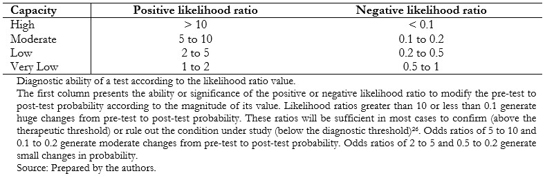
Positive likelihood ratios can have values between one and infinity and negative likelihood ratios between zero and one. A likelihood ratio of one indicates null utility for discriminating the presence or absence of a condition[23],[24],[25] (Table 1).

Table 1.

Diagnostic potency.

Full size

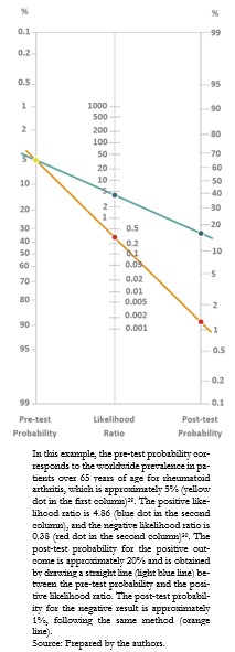
The most practical and straightforward way to interpret the likelihood ratios is by applying Bayes’ theorem with Fagan’s nomogram[27],[28]. In this graph, the left column represents the pre-test probability, the middle column the likelihood ratio of the diagnostic test applied and the right column the post-test probability[19]. By extending a straight line joining the values obtained from the first column with that of the second column, it is possible to obtain the result of the third column, corresponding to the probability of having the condition, by means of the diagnostic test result (Example 11).

Figure 6.

Fagan nomogram of rheumatoid factor.

Full size

A positive result for the rheumatoid factor, without other signs or symptoms supporting the presence of rheumatoid arthritis, is not sufficient to make the diagnosis, much less to justify treatment[31].

Receiver operating characteristic curve

Some diagnostic tests report their results in continuous or ordinal data, such as blood pressure or glycemia. The cut-off point where the highest sensitivity and specificity exists must be determined when using this type of data, i.e., the place on the curve where the sick are best discriminated from the healthy individuals[32]. However, no exact value separates the sick from the healthy, with overlapping values between the two groups.

Receiver operating characteristic curves are a graphical representation that relates the proportion of true positives (sensitivity) to the proportion of false positives (1 minus specificity) for different possible values of a diagnostic test to determine which value best discriminates between sick and healthy individuals. The receiver operating characteristic curve is constructed from a scatter plot, whose ordinate (y) and abscissa (x) axes correspond respectively to the sensitivity and the complement of the specificity for the different possible outcomes of the diagnostic test. A dotted line is drawn from the lower left corner and the upper right corner of the graph and is called the “reference diagonal” or “non-discrimination line”. This reference diagonal corresponds to the theoretical representation of a diagnostic test that does not discriminate between sick and healthy individuals (identical distribution of results for both groups).

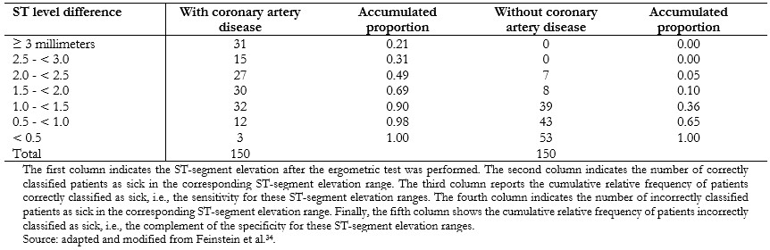
The cut-off point that discriminates best between sick and healthy within the receiver operating characteristic curve is the one that achieves the highest sensitivity and specificity at the same time. Graphically, it corresponds to the point closest to the upper left corner of the graph, calculated using the Youden index (sensitivity + specificity - 1)[33]. However, depending on the clinical objective of the diagnostic test, the cut-off point may be different to favor sensitivity or specificity (Example 12).

Table 2.

Values obtained in the ergometric test.

Full size

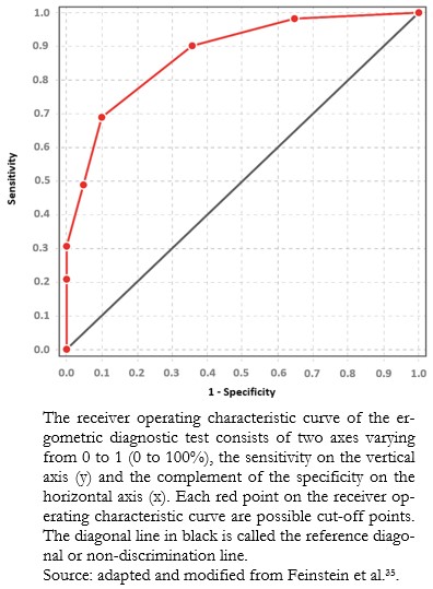
The cut-off point that best discriminates between healthy patients and patients with coronary artery disease for this diagnostic test would be the ST-segment elevation greater than or equal to 1.5 millimeters, which has a sensitivity of 0.69 and a specificity of 0.90. However, in clinical practice, the cut-off point used for coronary artery disease is ST-segment elevation greater than 1 millimeter, which has a sensitivity of 0.90 and a specificity of 0.64. This cut-off point privileges sensitivity at the expense of specificity[35],[36], since failure to diagnose coronary artery disease (false negative) can be harmful and even fatal for patients. The data obtained in this example are illustrated in a receiver operating characteristic curve (Figure 7).

Figure 7.

Operating characteristic curve of the ergometric test receiver.

Full size

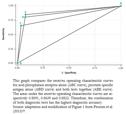
The area under the receiver operating characteristic curve is the global indicator of the accuracy of a diagnostic test, the calculation of which is beyond the scope of this study. This area ranges from 0.5 to 1. At 1, diagnostic tests achieve 100% sensitivity and specificity. An area close to 0.5 means that the diagnostic test cannot discriminate between sick and healthy patients. The area under the receiver operating characteristic curve allows comparisons between two or more diagnostic tests[37], choosing, in general terms, the one with the largest area as the one that best discriminates between sick and healthy patients (Example 12).

Figure 8.

Comparison of receiver operating characteristic curves.

Full size

Conclusions

Diagnostic tests assist clinical decision-making, and for their analysis, it is essential to understand their properties (sensitivity, specificity, predictive values, and likelihood ratios).

Following Bayes’ theorem, from the baseline probability of the individual (pre-test probability) and the properties of the test and its results, we can achieve a new probability for the condition under study.

Receiver operating characteristic curves are valuable tools for evaluating diagnostic tests with non-dichotomous quantitative results, allowing discrimination between two health states.

The correct interpretation of test results can avoid decision-making errors and negative consequences for those subjected to these tests.